Case study 2: a multi-pathogen system with multivalent vaccinaton (diphtheria and pertussis)
Source:vignettes/case_study_2_diphtheria_pertussis.Rmd
case_study_2_diphtheria_pertussis.Rmd1. Outline
Here, we will use the serosim package to generate a
cross-sectional serosurvey of a multi-pathogen system with multivalent
vaccination. The overall structure and principles discussed within this
case study are applicable to pathogen systems like measles, mumps, and
rubella with MMR vaccination or diphtheria, tetanus, and pertussis
system with DTP vaccination among many others. This simulation will
track natural infection to a generic pathogen A, natural infection to
pathogen B and bivalent vaccination with pathogen A and pathogen B
specific biomarkers for 100 individuals across a 10 year period. At the
end of the 10 year period, we will measure biomarker quantities against
both pathogen A specific biomarkers and pathogen B specific biomarkers
for all individuals as a cross-sectional sample. We will set up each of
the required arguments and models for runserosim in the
order outlined in the methods section of the paper.
This case study is built around diphtheria and pertussis and we are interested in tracking bivalent vaccination and both diphtheria and pertussis natural infection across a 10 year period. We will conduct a cross-sectional serological survey where we will use an ELISA kit to measure an individual’s diphtheria and pertussis IgG titer.
We will use published diphtheria and pertussis serological studies and any well characterized epidemiological and immunological characteristics of diphtheria and pertussis to parameterize our models wherever possible and make reasonable assumptions for other required model parameters wherever information is lacking.
We narrowed our search to diphtheria and pertussis serological studies conducted with ELISA IgG test kits that reported quantitative titers in comparable units. We did not conduct an extensive search of all diphtheria and pertussis studies in order to parameterize our models as it is beyond the scope of this case study. Our aim was to provide a simple example of how users can use the literature to inform required serosim inputs. Within each section below, we will briefly explain the rationale behind our selected model inputs. We caution users to conduct their own research into the models and associated parameters which best align with their disease system and biomarker test kits.
Load necessary packages:
2. Simulation settings
We will simulate monthly time steps across a 10 year period. Therefore, we will have 120 time steps. Note that these are arbitrary time steps which will need to be scaled to the right time resolution to match any time-based parameters used later on.
3. Population demography
For this case study, we are interested in tracking an individual’s
socioeconomic status, group (a proxy for location), birth and removal
time. We will use the generate_pop_demography function to
create the demography tibble needed for runserosim.
Note: the runserosim function, called later on only
requires a demography tibble with two columns (individuals and
times).
## Specify the number of individuals in the simulation
N<-100

## Pre-load the demography categories, values and distributions
## Specify options for each demography element and the distribution of each within the population
## We are interested in simulating a population where individuals have varying nutritional status and can reside in either of 2 locations
aux <- list("NS"=list("name"="NS","options"=c("low","medium","high"), "distribution"=c(0.3,0.3,0.4)),
            "Group"=list("name"="group","options"=c(1, 2), "distribution"=c(0.5,0.5)))


## Generate the population demography tibble
## Let's assume that individuals are removed from the population and set prob_removal to 0.2
demography <- generate_pop_demography(N, times, age_min=0, removal_min=1, removal_max=120, prob_removal=0.2, aux=aux)
## Joining with `by = join_by(i)`
## Examine the generated demography tibble
head(demography)
## # A tibble: 6 × 6
## i birth removal times NS group
## <int> <dbl> <dbl> <dbl> <chr> <dbl>
## 1 1 23 121 1 medium 2
## 2 1 23 121 2 medium 2
## 3 1 23 121 3 medium 2
## 4 1 23 121 4 medium 2
## 5 1 23 121 5 medium 2
## 6 1 23 121 6 medium 2
tail(demography)## # A tibble: 6 × 6
## i birth removal times NS group
## <int> <dbl> <dbl> <dbl> <chr> <dbl>
## 1 100 79 82 115 low 1
## 2 100 79 82 116 low 1
## 3 100 79 82 117 low 1
## 4 100 79 82 118 low 1
## 5 100 79 82 119 low 1
## 6 100 79 82 120 low 14. Exposure to biomarker mapping
We must set up the exposure IDs and biomarker IDs for our desired simulation. Individuals can be seropositive either by natural infection or by vaccination and we want to track both exposure types separately.
In this case, we need three exposure IDs:
- Diphtheria natural infection (
DP_ifxn) - Pertussis natural infection (
PT_ifxn) - Diphtheria and pertussis combined vaccination
(
vacc)
And two biomarker IDs:
- Diphtheria-specific biomarkers (
DP_antibody) - Pertussis-specific biomarkers (
PT_antibody)
runserosim requires that exposure_id and
biomarker_id are numeric, so we will use the
reformat_biomarker_map function to create a new version of
the biomarker map. Note that the reformat_biomarker_map
function will number the exposures and biomarkers in alphabetical order
so that the first exposure event or biomarker that is listed will not
necessarily be labeled as 1.
## Create biomarker map
biomarker_map_original <- tibble(exposure_id=c("DP_ifxn","PT_ifxn","vacc","vacc"),biomarker_id=c("DP_antibody","PT_antibody","DP_antibody","PT_antibody"))
biomarker_map_original
## # A tibble: 4 × 2
## exposure_id biomarker_id
## <chr> <chr>
## 1 DP_ifxn DP_antibody
## 2 PT_ifxn PT_antibody
## 3 vacc DP_antibody
## 4 vacc PT_antibody
## Reformat biomarker_map for runserosim
biomarker_map <-reformat_biomarker_map(biomarker_map_original)
biomarker_map
## # A tibble: 4 × 2
## exposure_id biomarker_id
## <dbl> <dbl>
## 1 1 1
## 2 2 2
## 3 3 1
## 4 3 25. Force of exposure and exposure model
Now, we need to specify the foe_pars argument which
contains the force of exposure for all exposure_IDs across all time
steps and groups. We also need to specify the exposure model which will
be called within runserosim later. The exposure model will
determine the probability that an individual is exposed to a specific
exposure event.
Here, we specified the same force of exposure for all time steps
within foe_pars for simplicity but users can input varying
values to match real world settings.
For our selected exposure model, the probability of exposure
(1-e^(-λ)) depends on the force of exposure (λ) at the current time
t for group g modulated by relevant demographic
elements (dem_mod). For simplicity, we selected arbitrary
age and demography modifiers specified below. Since we have two groups,
there are 2 rows in the first foe_pars dimension to specify
the group-specific force of exposure.
## Create an empty array to store the force of exposure for all exposure types across all time steps and groups
## Dimension 1: Group
## Dimension 2: Times
## Dimension 3: Exposure ID in the numeric order that they appear in the biomarker map
foe_pars <- array(0, dim=c(n_distinct(demography$group),max(times), n_distinct(biomarker_map$exposure_id)))

## Note that we can specify a different force of exposure for each group, time and exposure ID
## We specified the same value for all time steps within foe_pars for simplicity.

## Specify the force of exposure for exposure ID 1 which represents diphtheria natural infection (DP_ifxn)
foe_pars[1,,1] <- 0.04 ## Group 1 (aka Location 1)
foe_pars[2,,1] <- 0.03 ## Group 2 (aka Location 2)

## Specify the force of exposure for exposure ID 2 which represents pertussis natural infection (PT_ifxn)
foe_pars[1,,2] <- 0.02 ## Group 1 (aka Location 1)
foe_pars[2,,2] <- 0.01 ## Group 2 (aka Location 2)

## Specify the force of exposure for exposure ID 3 which represents diphtheria and pertussis combined vaccine (vacc)
foe_pars[1,,3] <- 0.02 ## Group 1 (aka Location 1)
foe_pars[2,,3] <- 0.03 ## Group 2 (aka Location 2)

## Specify a simple exposure model which calculates the probability of exposure from the force of exposure modulated by age and demography elements
exposure_model<-exposure_model_dem_mod

## This exposure model requires dem_mod and t_in_year arguments

## Create a tibble with any relevant demography modifiers that affect exposure probability
## For simplicity, we selected arbitrary numbers.

## First, we will specify age modifiers
## Individuals who are 0-3 are 2 times more likely to be exposed to diphtheria
age_mod_1<-tibble(exposure_id=rep(1,11), column=rep("age",times=11), value=0:10, modifier=c(2,2,2,2,1,1,1,1,1,1,1))

## Individuals who are 0-3 are 2 times more likely to be exposed to pertussis
age_mod_2<-tibble(exposure_id=rep(2,11), column=rep("age",times=11), value=0:10, modifier=c(2,2,2,1,1,1,1,1,1,1,1))

## Individuals who are less than one year old are 3 times more likely be vaccinated than other age classes
age_mod_3<-tibble(exposure_id=rep(3,11), column=rep("age",times=11),  value=0:10, modifier=c(3,1,1,1,1,1,1,1,1,1,1))
age_mod<-rbind(age_mod_1,age_mod_2,age_mod_3)
age_mod
## # A tibble: 33 × 4
## exposure_id column value modifier
## <dbl> <chr> <int> <dbl>
## 1 1 age 0 2
## 2 1 age 1 2
## 3 1 age 2 2
## 4 1 age 3 2
## 5 1 age 4 1
## 6 1 age 5 1
## 7 1 age 6 1
## 8 1 age 7 1
## 9 1 age 8 1
## 10 1 age 9 1
## # ℹ 23 more rows
## Now we will  specify additional demography exposure modifiers and combine them with the previous ones
## Here, individuals who are of low nutritional status are twice as likely of being exposed to diphtheria and pertussis while individuals who are of medium nutritional status are 1.5 times as likely of being exposed when compared to individuals of high nutritional status
## Individuals of high nutritional status are 3 times more likely to be exposed to exposure ID 3 (vaccination) while individuals who are of medium nutritional status are 2 times more likely to be exposed to exposure ID 3 (vaccination) than individuals of low nutritional status.
## Note that the modifiers must be defined for all combinations of exposure types and demographic elements
mod<-tibble(exposure_id=c(1,1,1,2,2,2,3,3,3), column=rep("NS",times=9), value=rep(c("low","medium", "high"),3), modifier=c(2,1.5,1,2,1.5,1,1,2,3))
mod
## # A tibble: 9 × 4
## exposure_id column value modifier
## <dbl> <chr> <chr> <dbl>
## 1 1 NS low 2
## 2 1 NS medium 1.5
## 3 1 NS high 1
## 4 2 NS low 2
## 5 2 NS medium 1.5
## 6 2 NS high 1
## 7 3 NS low 1
## 8 3 NS medium 2
## 9 3 NS high 3
## Combine both age modifiers and additional modifiers
dem_mod<-rbind(age_mod,mod)

## Specify the number of time steps within a year which will be used to calculate an individual's age.
## We are simulating on the monthly scale so there are 12 time steps within a year.
t_in_year=12

## Examine the probability of exposure over time for the specified exposure model
plot_exposure_model(indivs=1:5,exposure_model=exposure_model_dem_mod, times=times, n_groups = 2, n_exposures = 3, foe_pars=foe_pars, demography=demography, dem_mod=dem_mod,t_in_year=t_in_year)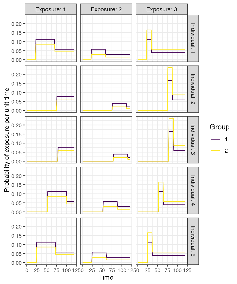
6. Immunity model
Next, we specify the immunity model which will determine the
probability that an exposure event is successful in inducing an
immunological response. Since we have both vaccination and natural
infection events, we will use
immunity_model_vacc_ifxn_biomarker_prot. With this immunity
model, the probability of successful vaccination exposure depends on the
number of vaccines received prior to time t and the
individual’s age at time t, while the probability of successful
infection is dependent on the biomarker quantity, in this case antibody
titer, at the time of exposure. Individuals can have up to 3 successful
vaccination events (aka 3 doses) and are eligible for vaccination
starting at 2 months of age to align with the diphtheria/pertussis
vaccination schedule.
We placed no limit on the maximum number of infections to either
diphtheria or pertussis however our selected immunity model will take
into account an individual’s current biomarker
level when determining the probability of a successful infection.
Additional successful exposure events (reinfection) events are
representative of boosting events which can occur if an individual is
exposed to either pathogen following a vaccination or previous
infection. The user can limit the frequency of reinfections by adjusting
the biomarker-mediated protection (also known as titer-mediated
protection or titer-ceiling effects) parameters or by specifying a
maximum number of allowed successful exposure events. The titer-mediated
protection parameters used within this model are defined within
model_pars which will be loaded in section 6.
Again, the following diphtheria and pertussis titer-mediated protection parameters were selected by a literature search. The titer cutoffs used below were also discussed in a previous analysis of diphtheria and pertussis serology (Razafimahatratra et al. 2022).
Diphtheria: 1. Individuals whose diphtheria antibody levels under 0.01 IU/mL are considered highly susceptible to disease while individuals with higher levels are associated with less severe symptoms (Ipsen 1946; Björkholm et al. 1986; Danilova et al. 2006; Ohuabunwo et al. 2005). 2. Individuals whose antibody levels are 0.01 IU/mL have the lowest titer level which confers some degree of protection while individuals with >=0.1 IU/mL are associated with long term protection (Efstratiou, Maple, and World Health Organization. Regional Office for Europe 1994,). 3. Antibody levels in between 0.01 and 0.09 IU/mL are considered to provide basic levels of protection against disease (World Health Organization 2017).
Pertussis: 1. Low anti-pertussis IgG antibodies have shown significant correlation with pertussis susceptibility (Storsaeter et al. 2003) but a protective threshold has not been established (Saso and Kampmann 2020) since there is no established immunological correlate of protection against disease (Plotkin 2008). 2. Given the information presented above, we have chosen that antibody levels between 40-100 IU/mL will confer higher level of protection since they are indicative of serpositivity and of recent pertussis infection or pertussis vaccination (“BORDG - Overview: Bordetella Pertussis Antibody, IgG, Serum,” n.d.; Chen et al. 2016).
## Specify immunity model within the runserosim function below
immunity_model<-immunity_model_vacc_ifxn_biomarker_prot

## Specify which exposure IDs represent vaccination events
## In this case, only exposure ID 3 is a vaccination event
vacc_exposures<-3

## Specify the time step after birth at which an individual is eligible for vaccination (2 months old for diphtheria and pertussis combine vaccine); ; note non-vaccine exposures are listed as NAs
vacc_age<-c(NA,NA,2)

## Specify the maximum number of successful exposure events an individual can receive for each exposure type
## We placed no successful exposure limit on the number of diphtheria or pertussis infection exposures and 3 dose limit on the vaccine exposure.
max_events<-c(Inf,Inf,3)

## Plot biomarker-mediated protection curve given parameters specified within model_pars for biomarker 1, diphtheria antibody  (DP_antibody) which will be loaded in section 6
## The immunity model we selected will take into account an individual's current titer to diphtheria when determining the probability of successful infection.
## Titers are ploted in mIU/mL
plot_biomarker_mediated_protection(0:150, biomarker_prot_midpoint=75, biomarker_prot_width=.1)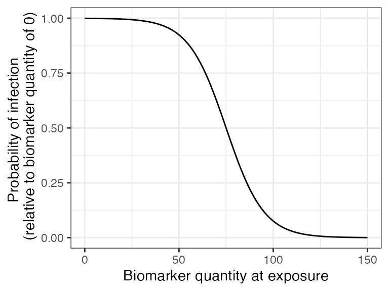
## Plot biomarker-mediated protection curve given parameters specified within model_pars for biomarker 2, pertussis antibody (PT_antibody) which will be loaded in section 6
## The immunity model we selected will take into account an individual's current titer to pertussis when determining the probability of successful infection.
## Titers are ploted in IU/mL
plot_biomarker_mediated_protection(0:100, biomarker_prot_midpoint=40, biomarker_prot_width=.25)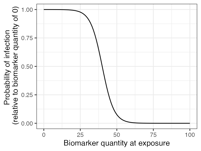
7. Antibody model and model parameters
Now, we specify the antibody model to be used within
runserosim to track antibody kinetics, or more broadly
biomarker kinetics for each biomarker produced from successful exposure
events. We will use a biphasic boosting-waning model(Voysey et al. 2016). This model assumes
that for each exposure there is a set of long-term boost, long-term
waning, short-term boost, and short-term waning parameters.
The antibody kinetics parameters needed for the antibody model are
pre-loaded within a csv file which will take on the argument name:
model_pars. Users can edit the csv file to modify any
parameters or change the parameters in R. runserosim
requires that exposure_id and biomarker_id are
numeric within model_pars so we will use the
reformat_biomarker_map function again to create a new
version of model_pars. Users defining their own
model_pars table could set the exposure_id and
biomarker_id as numeric in the first place if
preferred.
We selected a few diphtheria and pertussis serological surveys conducted which reported IgG titers following vaccination to inform the vaccine induced boost and waning parameters. There are many complexities and heterogeneity in these parameters which arise from different vaccine types and vaccination schedules. We attempt to simplify these complexities and select a few papers to give us some rough parameters for this example simulation.
After 3 vaccine doses, diphtheria titers ranged from 1.5-1.7 IU/mL (Kimura et al. 1991) and pertussis titers above 100 IU/mL were associated with recent vaccination (“BORDG - Overview: Bordetella Pertussis Antibody, IgG, Serum,” n.d.). Diphtheria antibody half-life has been estimated to be around 19-27 years (Amanna, Carlson, and Slifka 2007; Hammarlund et al. 2016) with 10% of children losing immunity by one year following the primary vaccination series (Pichichero et al. 1987); 67% of children after 3 to 13 years and 83% after 14 to 23 years (Crossley et al. 1979). As for pertussis, the duration of immunity after a 3 dose series of the wP vaccine is estimated to be from 4 to 12 years (Sheridan et al. 2014). Pertussis titers >=100 IU/mL are associated with recent infection or vaccination within the past year while titers between 40 and 100 IU/mL are associated with recent infection (“BORDG - Overview: Bordetella Pertussis Antibody, IgG, Serum,” n.d.)
Our selected antibody kinetics parameters given our brief and limited literature search are as follows:
Diphtheria vaccine:
- Long term boost: 0.3-0.5 IU/mL
- Long term waning: 0.01 IU/mL per month
- Short term boost: 0.1-0.3 IU/mL
- Short term waning: 0.033 IU/mL per month
Pertussis vaccine:
- Long term boost: 30-50 IU/mL
- Long term waning: 0.0066 IU/mL per month
- Short term boost: 40-80 IU/mL
- Short term waning: 0.016 IU/mL per month
We were unable to find studies that reported titer kinetics following known infection events in comparable units. For simplicity, we will assume that natural infection boosting parameters are 25% higher than vaccine induced antibody boosting with similar waning rates.
Lastly, we define the draw_parameters function which
determines how each individual’s antibody kinetics parameters are
simulated from the within-host processes parameters tibble
(model_pars). We will use a function which draws parameters
directly from model_pars for the antibody model with random
effects to represent individual heterogeneity in immunological
responses. Parameters are drawn randomly from a distribution with mean
and standard deviation specified within model_pars. This
draw_parameters function also incorporates biomarker
quantitiy dependent boosting, where an individual’s realized boost is
dependent on their titer level at the time of the exposure event.
We arbitrarily set the diphtheria titer-dependent boosting effects following an additional successful exposure event for individuals with diphtheria levels above 1.7 IU/mL to be only 10% of the full boost. Similarly, individuals with pertussis titers above 100 IU/mL will only receive 10% of the full boost for any additional successful exposure event.
## Specify the antibody model
antibody_model<-antibody_model_biphasic

## Bring in the antibody parameters needed for the antibody model
## Note that the titer-mediated protection parameters needed for the immunity model, the titer-ceiling parameters needed for draw_parameters and the observation error parameter needed for the observation model are all defined here too.
## Also note that these are all arbitrary parameter values chosen for this toy example.
model_pars_path <- system.file("extdata", "model_pars_cs2.csv", package = "serosim")
model_pars_original <- read.csv(file = model_pars_path, header = TRUE)
model_pars_original
## exposure_id biomarker_id name mean sd
## 1 vacc DP_antibody boost_long 0.400000 1e-01
## 2 vacc DP_antibody boost_short 0.200000 1e-01
## 3 vacc DP_antibody wane_long 0.010000 5e-03
## 4 vacc DP_antibody wane_short 0.033000 5e-03
## 5 vacc DP_antibody biomarker_ceiling_threshold 1.700000 NA
## 6 vacc DP_antibody biomarker_ceiling_gradient 0.529411 NA
## 7 <NA> DP_antibody obs_sd NA 5e-02
## 8 vacc PT_antibody boost_long 40.000000 1e+01
## 9 vacc PT_antibody boost_short 60.000000 2e+01
## 10 vacc PT_antibody wane_long 0.006600 5e-04
## 11 vacc PT_antibody wane_short 0.016000 5e-04
## 12 vacc PT_antibody biomarker_ceiling_threshold 100.000000 NA
## 13 vacc PT_antibody biomarker_ceiling_gradient 0.009000 NA
## 14 <NA> PT_antibody obs_sd NA 1e+01
## 15 DP_ifxn DP_antibody boost_long 0.500000 1e-01
## 16 DP_ifxn DP_antibody boost_short 0.250000 1e-01
## 17 DP_ifxn DP_antibody wane_long 0.010000 5e-03
## 18 DP_ifxn DP_antibody wane_short 0.033000 5e-03
## 19 DP_ifxn DP_antibody biomarker_ceiling_threshold 1.700000 NA
## 20 DP_ifxn DP_antibody biomarker_ceiling_gradient 0.529411 NA
## 21 DP_ifxn DP_antibody biomarker_prot_midpoint 0.075000 NA
## 22 DP_ifxn DP_antibody biomarker_prot_width 0.100000 NA
## 23 PT_ifxn PT_antibody boost_long 50.000000 1e+01
## 24 PT_ifxn PT_antibody boost_short 75.000000 2e+01
## 25 PT_ifxn PT_antibody wane_long 0.006600 5e-04
## 26 PT_ifxn PT_antibody wane_short 0.016000 5e-04
## 27 PT_ifxn PT_antibody biomarker_ceiling_threshold 100.000000 NA
## 28 PT_ifxn PT_antibody biomarker_ceiling_gradient 0.009000 NA
## 29 PT_ifxn PT_antibody biomarker_prot_midpoint 40.000000 NA
## 30 PT_ifxn PT_antibody biomarker_prot_width 0.250000 NA
## distribution
## 1 log-normal
## 2 log-normal
## 3 log-normal
## 4 log-normal
## 5
## 6
## 7 normal
## 8 log-normal
## 9 log-normal
## 10 log-normal
## 11 log-normal
## 12
## 13
## 14 normal
## 15 log-normal
## 16 log-normal
## 17 log-normal
## 18 log-normal
## 19
## 20
## 21
## 22
## 23 log-normal
## 24 log-normal
## 25 log-normal
## 26 log-normal
## 27
## 28
## 29
## 30
## Reformat model_pars for runserosim
model_pars<-reformat_biomarker_map(model_pars_original)
model_pars
## exposure_id biomarker_id name mean sd
## 1 3 1 boost_long 0.400000 1e-01
## 2 3 1 boost_short 0.200000 1e-01
## 3 3 1 wane_long 0.010000 5e-03
## 4 3 1 wane_short 0.033000 5e-03
## 5 3 1 biomarker_ceiling_threshold 1.700000 NA
## 6 3 1 biomarker_ceiling_gradient 0.529411 NA
## 7 NA 1 obs_sd NA 5e-02
## 8 3 2 boost_long 40.000000 1e+01
## 9 3 2 boost_short 60.000000 2e+01
## 10 3 2 wane_long 0.006600 5e-04
## 11 3 2 wane_short 0.016000 5e-04
## 12 3 2 biomarker_ceiling_threshold 100.000000 NA
## 13 3 2 biomarker_ceiling_gradient 0.009000 NA
## 14 NA 2 obs_sd NA 1e+01
## 15 1 1 boost_long 0.500000 1e-01
## 16 1 1 boost_short 0.250000 1e-01
## 17 1 1 wane_long 0.010000 5e-03
## 18 1 1 wane_short 0.033000 5e-03
## 19 1 1 biomarker_ceiling_threshold 1.700000 NA
## 20 1 1 biomarker_ceiling_gradient 0.529411 NA
## 21 1 1 biomarker_prot_midpoint 0.075000 NA
## 22 1 1 biomarker_prot_width 0.100000 NA
## 23 2 2 boost_long 50.000000 1e+01
## 24 2 2 boost_short 75.000000 2e+01
## 25 2 2 wane_long 0.006600 5e-04
## 26 2 2 wane_short 0.016000 5e-04
## 27 2 2 biomarker_ceiling_threshold 100.000000 NA
## 28 2 2 biomarker_ceiling_gradient 0.009000 NA
## 29 2 2 biomarker_prot_midpoint 40.000000 NA
## 30 2 2 biomarker_prot_width 0.250000 NA
## distribution
## 1 log-normal
## 2 log-normal
## 3 log-normal
## 4 log-normal
## 5
## 6
## 7 normal
## 8 log-normal
## 9 log-normal
## 10 log-normal
## 11 log-normal
## 12
## 13
## 14 normal
## 15 log-normal
## 16 log-normal
## 17 log-normal
## 18 log-normal
## 19
## 20
## 21
## 22
## 23 log-normal
## 24 log-normal
## 25 log-normal
## 26 log-normal
## 27
## 28
## 29
## 30
## Specify the draw_parameters function to use
draw_parameters<-draw_parameters_random_fx_biomarker_dep
## Plot biomarker (in this case antibody titer) dependent boosting effects given parameters specified within model_pars for biomarker 1, diphtheria antibody (DP_antibody)
plot_biomarker_dependent_boosting(start=0, end=2, by=.1, biomarker_ceiling_threshold=1.7, biomarker_ceiling_gradient=0.529411)
## Plot biomarker (in this case antibody titer) dependent boosting effects given parameters specified within model_pars for biomarker 2, pertussis antibody (PT_antibody)
plot_biomarker_dependent_boosting(start=0, end=125, by=1, biomarker_ceiling_threshold=100, biomarker_ceiling_gradient=0.009)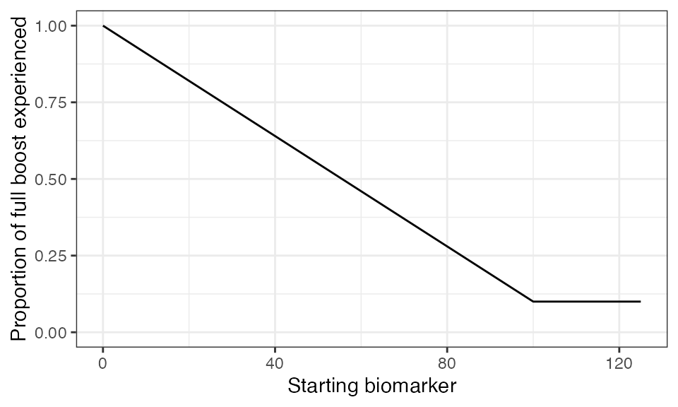
## Plot example biomarker trajectories given the specified antibody kinetics model, model parameters and draw parameters function
plot_antibody_model(antibody_model_biphasic, N=25, model_pars=model_pars,draw_parameters_fn = draw_parameters_random_fx_biomarker_dep, biomarker_map=biomarker_map) + scale_color_viridis_d()
## Scale for colour is already present.
## Adding another scale for colour, which will replace the existing scale.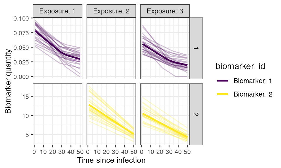
8. Observation model
Now we specify how observed biomarker quantities, in this case antibody titers, are generated as a probabilistic function of the true, latent biomarker quantities, and when to observe these quantities. In this step, users are specifying the sampling design and assay choice for their serological study.
This observation model observes the latent titer values given a
continuous assay with user-specified lower and upper limits, and added
measurement noise. The added noise represents assay variability and is
done by sampling from a distribution with the latent antibody titer as
the mean and the measurement error as the standard deviation. The
observation standard deviation and distribution is defined within
model_pars as the obs_sd parameter for each biomarker.
Diphtheria:
- Lower limit of ELISA IgG Detectability: 0.01 IU/mL
- Upper limit of ELISA IgG Detectability: 2 IU/mL
Pertussis:
- Lower limit of ELISA IgG Detectability: 5 IU/mL
- Upper limit of ELISA IgG Detectability: 200 IU/mL
## Specify the limits of detection for each biomarker for the continuous assays
bounds<-tibble(biomarker_id=c(1,1,2,2),name=rep(c("lower_bound","upper_bound"),2),value=c(0.01,2,5,200))

## Specify the observation model
observation_model<-observation_model_continuous_bounded_noise

## Specify observation_times to observe both biomarkers (aka DP_antibody and PT_antibody titers) across all individuals at the end of the simulation (t=120)
obs1 <- tibble(i=1:N,t=120, b=1)
obs2 <- tibble(i=1:N,t=120, b=2)
observation_times<-rbind(obs1,obs2)10. Run simulation
This is the core simulation where all simulation settings, models and parameters are specified within the main simulation function. The run time for this step varies depending on the number of individuals and the complexities of the specified models.
One way to speed up runserosim is to use the
attempt_precomputation flag. If set to true,
runserosim attempts to group interchangeable individuals in
the simulation, and vectorizes and pre-computes as many of the model
functions as possible. This can lead to considerable speed ups, but is
only usable for models with minimal dependency on intermediate states
(for example, it will not work if exposure probability is conditional on
a demography variable which changes over time). In any case,
serosim will detect this automatically, and will only use
the precomputed values if it a) provides a tangible speed up and b) does
not introduce errors into the model. We set
attempt_precomputation to false here, as the exposure
probability depends on individual-level demographic information which
can change during the simulation. It is also possible to use
parallelization with the parallel and foreach
package within runserosim by setting the
parallel argument to true and specifying the desired number
of cores.
res<- runserosim(
  simulation_settings,
  demography,
  observation_times,
  foe_pars,
  biomarker_map,
  model_pars,
  exposure_model,
  immunity_model,
  antibody_model,
  observation_model,
  draw_parameters,

  ## Other arguments needed
  bounds=bounds,
  max_events=max_events,
  vacc_exposures=vacc_exposures,
  vacc_age=vacc_age,
  dem_mod=dem_mod,
  t_in_year=t_in_year,
  VERBOSE=NULL,
  attempt_precomputation = FALSE
)
## Note that models and arguments specified earlier in the code can be specified directly within this function.
11. Generate plots
Now that the simulation is complete, we can examine the ground-truth states of the simulation for individual immune histories, the probability of exposure with each pathogen and vaccination over time, and the true, hidden biomarker kinetics.
## Plot biomarker 1 kinetics and immune histories for 10 individuals
plot_subset_individuals_history(res$biomarker_states %>% filter(b == 1), res$immune_histories_long, subset=10, demography, removal=TRUE)
## Warning: Removed 101 rows containing missing values (`geom_line()`).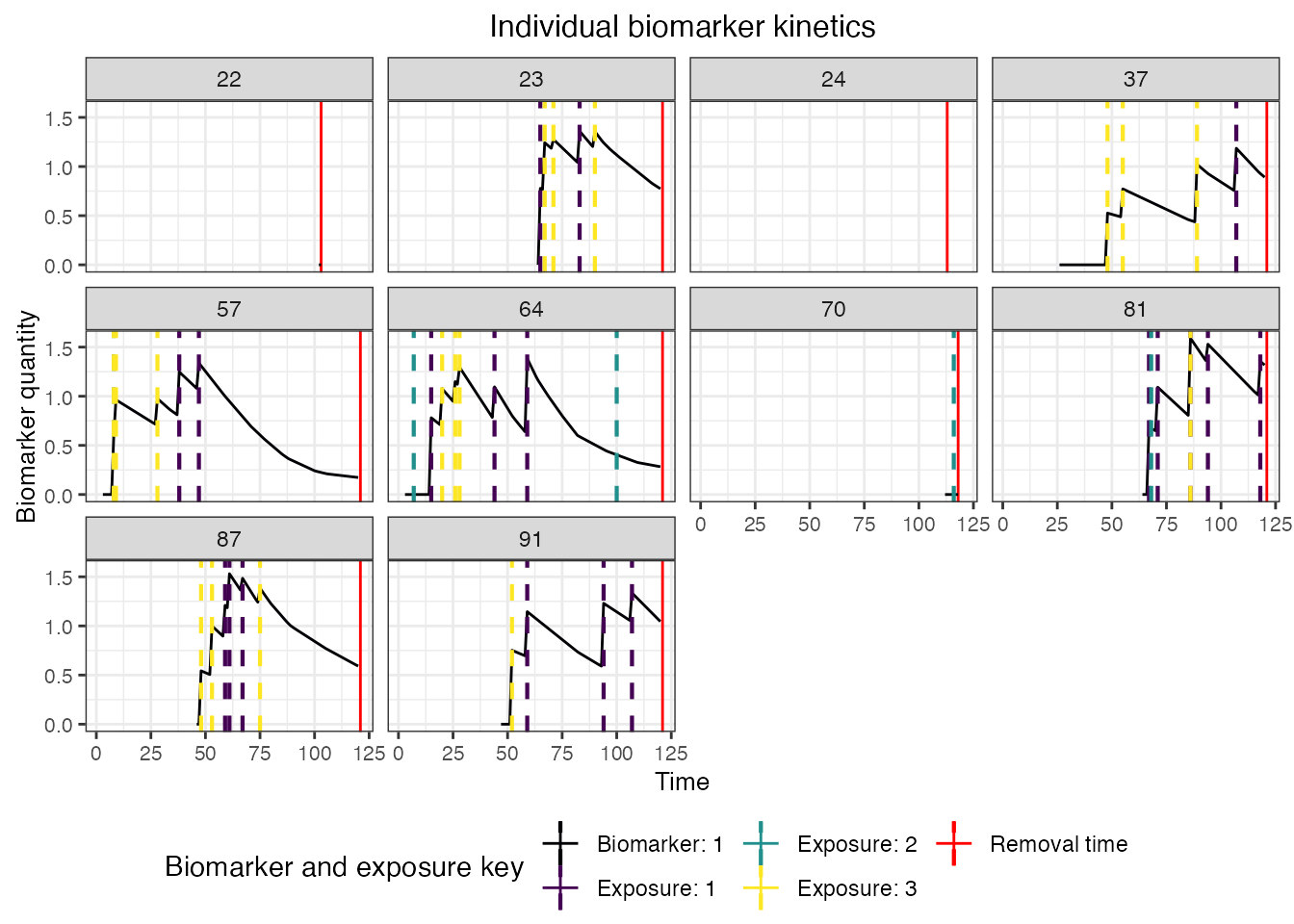
## Plot biomarker 2 kinetics and immune histories for 10 individuals
plot_subset_individuals_history(res$biomarker_states %>% filter(b == 2), res$immune_histories_long, subset=10, demography, removal=TRUE)
## Warning: Removed 48 rows containing missing values (`geom_line()`).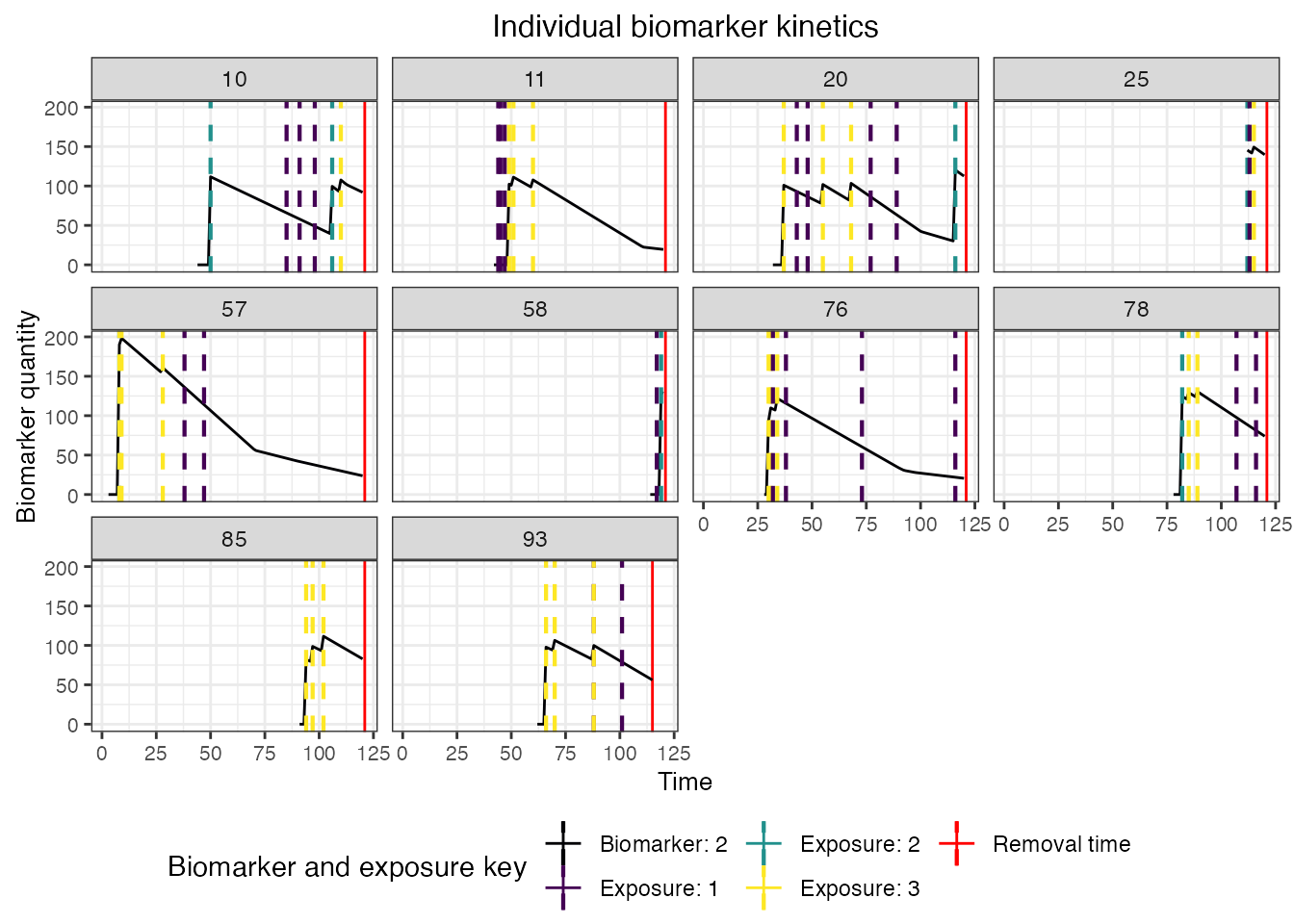
## Plot individual probability of exposure for all exposure types.
## This is the output of the exposure model.
plot_exposure_force(res$exposure_force_long)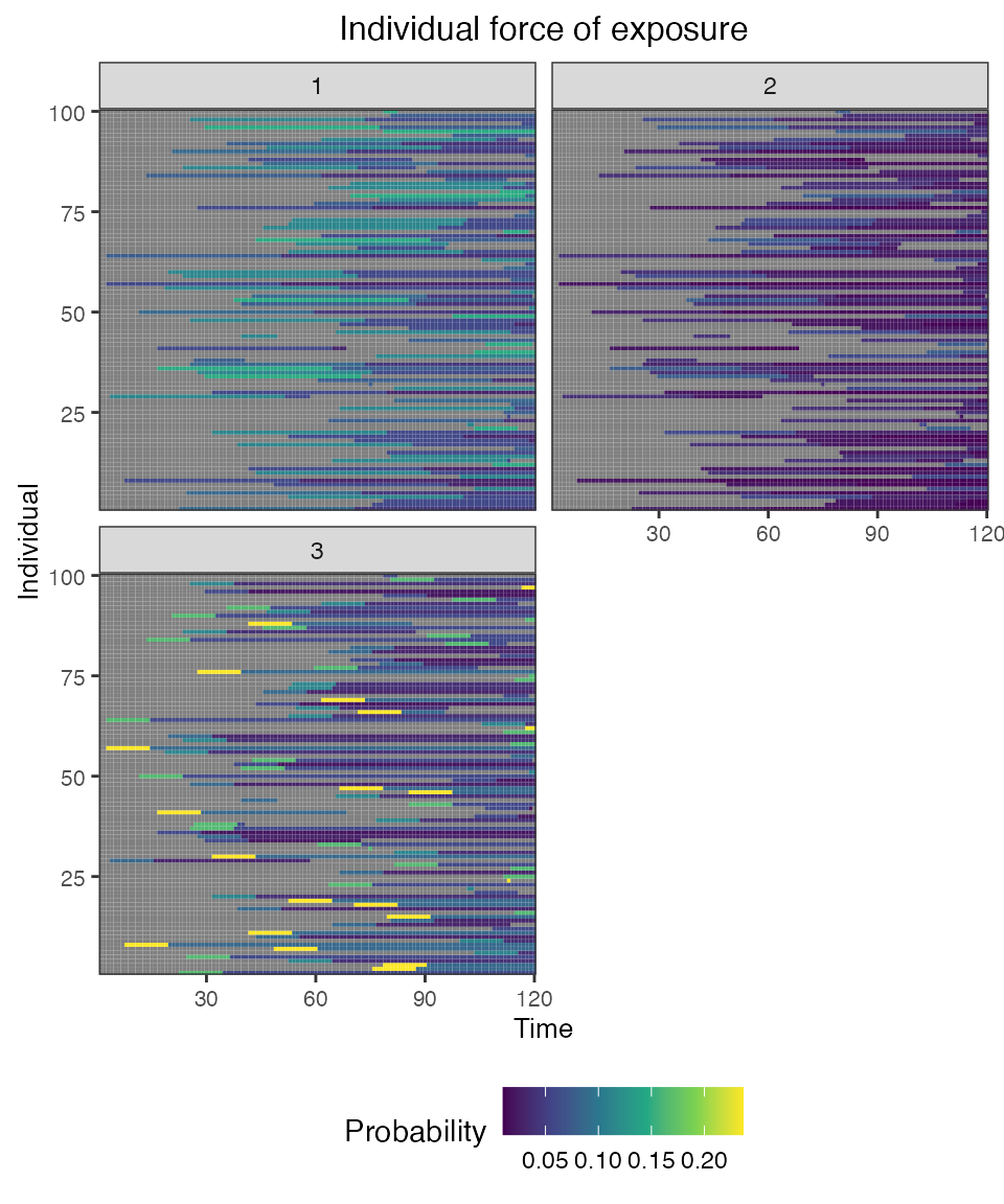
## Plot individual successful exposure probabilities for all exposure types
## This is the output of the exposure model multiplied by the output of the immunity model.
## In other words, this is the probability of exposure event being successful and inducing an immunological response
plot_exposure_prob(res$exposure_probabilities_long)
## Plot individual immune histories for all exposure types
plot_immune_histories(res$immune_histories_long)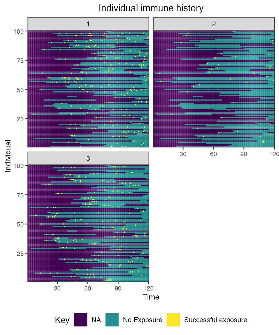
## Plot diphtheria and pertussis antibody states for all individuals (true biomarker quantities)
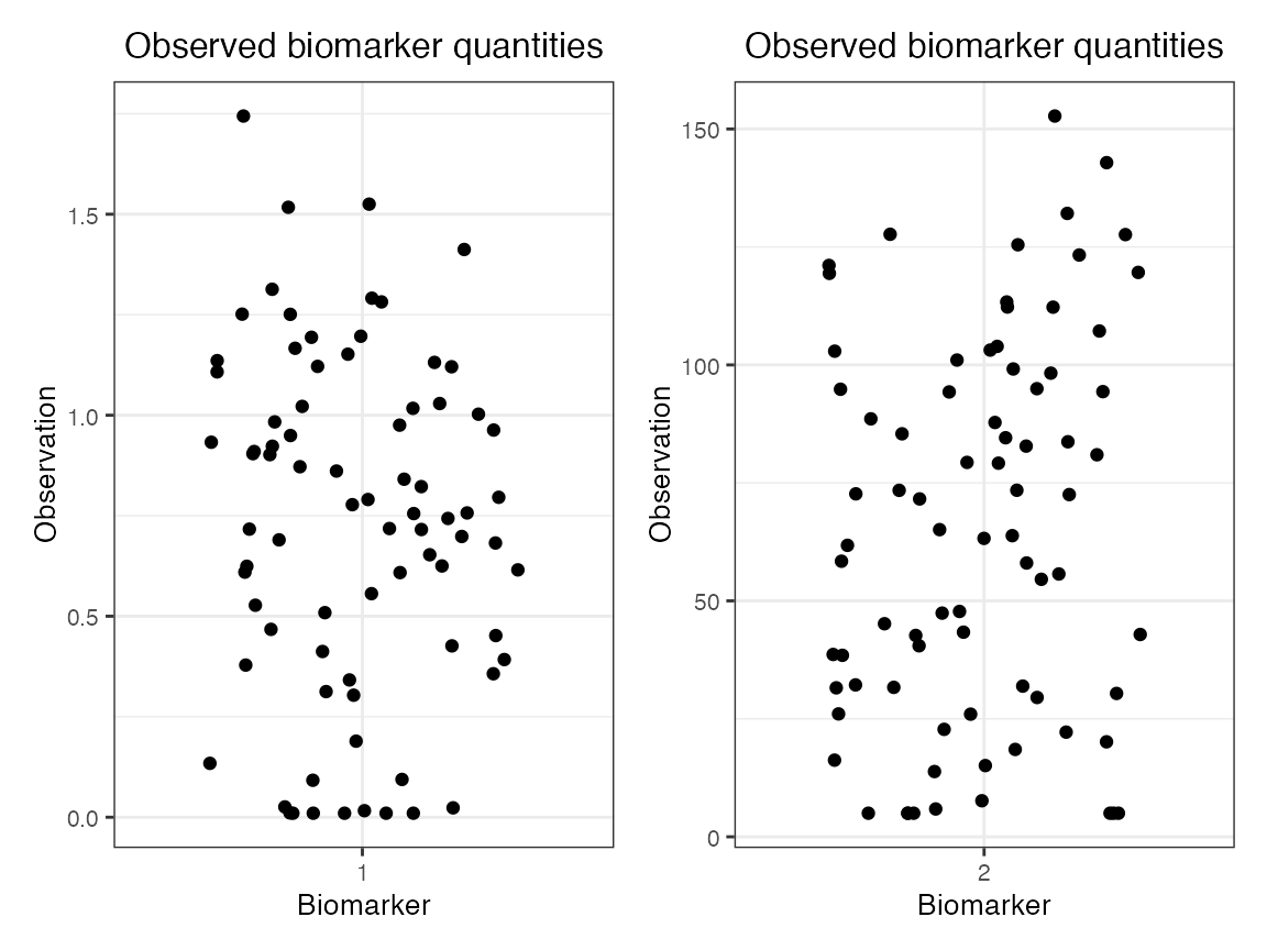
plot_biomarker_quantity(res$biomarker_states)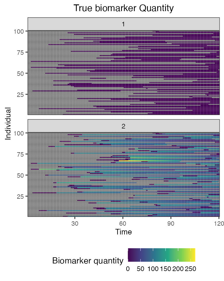 Finally, we can plot the simulate output of our cross-sectional
serosurvey. We use different plots due to the drastically different
scales of the two biomarkers.
Finally, we can plot the simulate output of our cross-sectional
serosurvey. We use different plots due to the drastically different
scales of the two biomarkers.
## Plot the diphtheria and pertussis serosurvey results (observed biomarker quantities)
plot_obs_biomarkers_one_sample(res$observed_biomarker_states %>% filter(b == 1)) | plot_obs_biomarkers_one_sample(res$observed_biomarker_states %>% filter(b == 2))