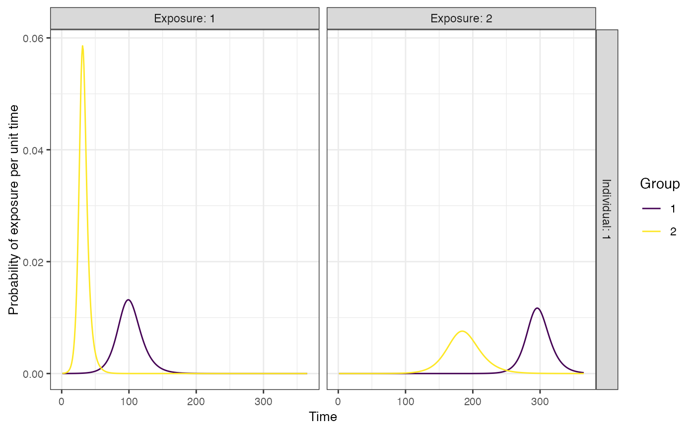
Plots the probability of exposure over time for the provided exposure models

plot_exposure_model(
  indivs = 1,
  exposure_model,
  times,
  n_groups = 1,
  n_exposures = 1,
  foe_pars,
  demography = NULL,
  ...
)

Arguments

indivs: (optional) vector of individuals to plot exposure probabilities for. This is important if the demography table contains information on more individuals than you wish to plot
exposure_model: A function calculating the probability of exposure given the foe_pars array
times: Vector of times to solve model over
n_groups: Number of groups corresponding to foe_pars
n_exposures: Number of exposure types corresponding to foe_pars
foe_pars: Generic object containing all parameters needed to solve exposure_model
demography: A tibble of demographic information for each individual in the simulation. At a minimum this tibble requires 1 column (i) where all individuals in the simulation are listed by row. This is used to calculate the sample population size. Additional variables can be added by the user, e.g., birth and removal times, see generate_pop_demography If not specified, the model will assume that birth time is the initial time point and removal time is the final time point across all individuals
...: Any additional arguments needed for the models

Value

A ggplot2 object

Examples

## Basic exposure model with demography modifier
times <- seq(1,120,1)
n_groups <- 1
n_exposures <- 2
foe_pars <- array(NA, dim=c(n_groups,length(times),n_exposures))
foe_pars[1,,1] <- 0.01
foe_pars[1,,2] <- 0.005 
aux <- list("SES"=list("name"="SES","options"=c("low","high"), "distribution"=c(0.5,0.5)))
demography <- generate_pop_demography(N=5, times, age_min=0, removal_min=1, 
removal_max=120, prob_removal=0.2, aux=aux)
#> Joining with `by = join_by(i)`
dem_mod <- dplyr::tibble(exposure_id=c(1,1,2,2),column=c("SES","SES","SES","SES"),
                 value=c("low","high","low","high"),modifier=c(1,0.75,1,0.5))

plot_exposure_model(indivs=1:5, exposure_model=exposure_model_dem_mod, 
times=times,1,2,foe_pars=foe_pars,demography = demography,dem_mod=dem_mod)

                    
## SIR model with two groups and two exposure types                 
foe_pars <- dplyr::bind_rows(
                      dplyr::tibble(x=1,g=1,name=c("beta","gamma","I0","R0","t0"),
                      value=c(0.3,0.2,0.00001,0,0)),
                      dplyr::tibble(x=2,g=1,name=c("beta","gamma","I0","R0","t0"),
                      value=c(0.35,0.25,0.00001,0,200)),
                      dplyr::tibble(x=1,g=2,name=c("beta","gamma","I0","R0","t0"),
                      value=c(0.5,0.2,0.00005,0,0)),
                      dplyr::tibble(x=2,g=2,name=c("beta","gamma","I0","R0","t0"),
                      value=c(0.27,0.2,0.00001,0,50))
                      )
plot_exposure_model(exposure_model=exposure_model_sir, times=seq(1,365,by=1),
n_groups = 2,n_exposures = 2,foe_pars=foe_pars)