A population trajectory applies the fitted covariate effects but excludes participant random effects. It therefore represents the latent kinetics for a specified population profile, not the arithmetic average of observed people.
prediction_grid(fit)

population <- predict(
  fit,
  type = "population",
  times = 0:150
)
plot(population)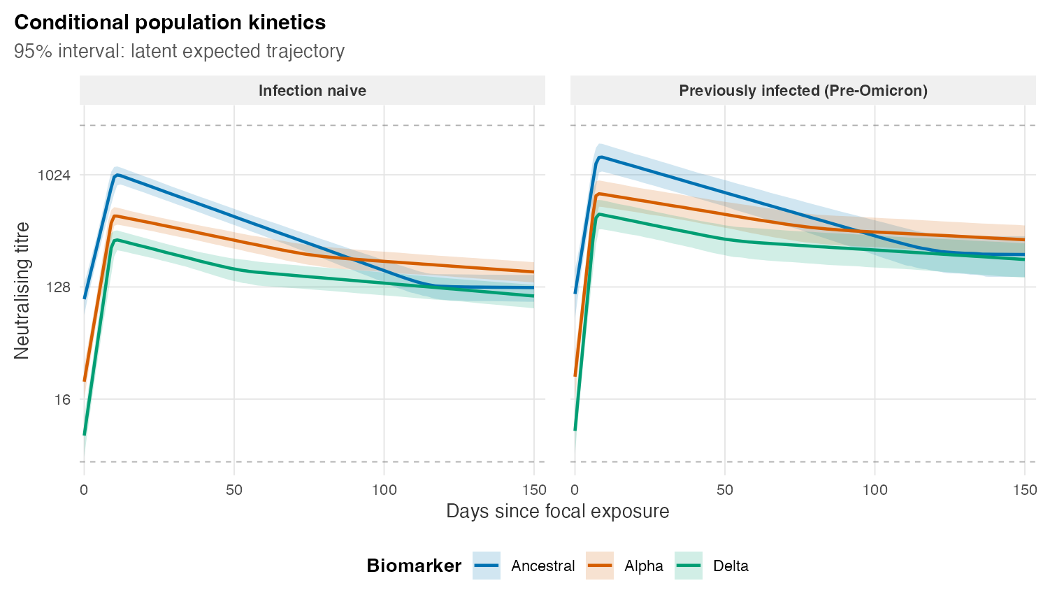
Conditional population trajectories from an actual package fit. Biomarkers share each panel and covariate profiles define facets. The line is the posterior median latent trajectory; ribbons are pointwise 95% credible intervals and dashed lines are censoring limits.
Prediction profiles
With newdata = NULL, prediction_grid()
keeps observed combinations of categorical predictors and fixes
continuous predictors at participant-level medians. This avoids silently
predicting impossible factor combinations.
profiles <- data.frame(
  infection_history = c(
    "Infection naive",
    "Previously infected (Pre-Omicron)"
  )
)

population <- predict(
  fit,
  type = "population",
  newdata = profiles,
  times = seq(0, 180, by = 2)
)
The stored formula terms, factor levels, contrasts, interactions, and
transformations create the new model matrix. Unknown levels fail early.
prediction_grid(fit, categorical = "cartesian")
deliberately requests every fitted-level combination when such
extrapolation is scientifically meaningful.
Summaries and uncertainty
Summarised output contains mean, median,
lower, and upper, plus time, biomarker, and
original profile columns. The plotting method uses the median by
default; plot(population, central = "mean") selects the
mean.
The default interval is uncertainty in the latent expected
trajectory. Set include_observation_noise = TRUE for a
posterior predictive interval for a future measured value; the returned
object and plot subtitle label this different target explicitly.
Use summary = FALSE to retain .draw and one
trajectory value per posterior draw. Preserve that identifier when
calculating joint quantities over times or biomarkers.
Response-scale output is the default. It uses log2-spaced axes with
natural response labels, matching the multiplicative outcome scale
without compressing the fitted curves. Every plotting method returns an
ordinary ggplot object.
Continue with Individual-level kinetics to add fitted participant effects and observations.