Covariates

Covariates describe systematic differences between participant profiles. They shift population kinetic parameters; participant random effects then describe remaining heterogeneity around those conditional population curves.

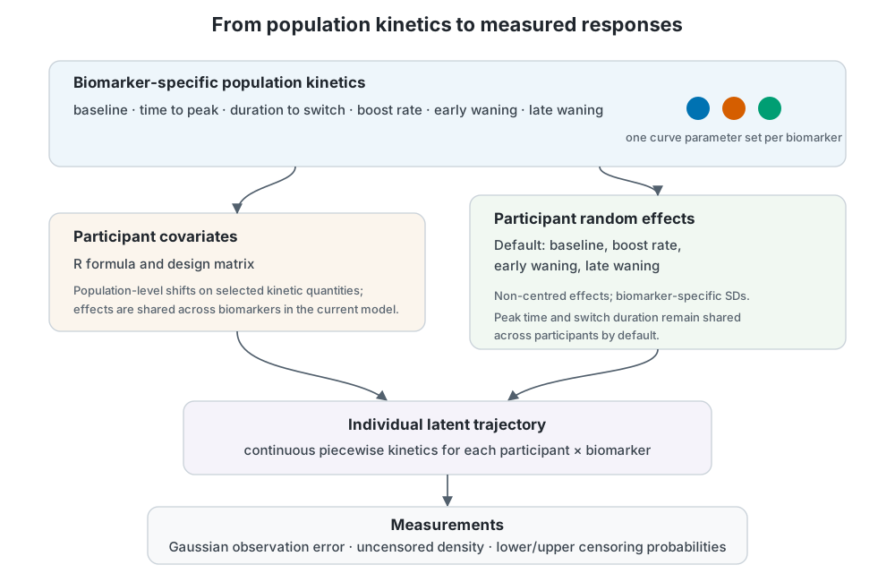
The default hierarchy. Biomarker-specific population kinetics are modified by participant covariates and selected non-centred participant effects, producing individual latent trajectories and finally measured or censored observations.

Formula and model matrix

Use an ordinary one-sided R formula:

library(epikinetics)
dat <- doc_delta_data()

prepared <- prepare_epikinetics_data(
  dat,
  formula = ~ infection_history,
  lower_limit = 5,
  upper_limit = 2560
)

prepared$mappings$reference_levels

#> infection_history 
#> "Infection naive"

prepared$mappings$design_columns

#>                                        design_column              term
#> 1 infection_historyPreviously infected (Pre-Omicron) infection_history
#>           variables                             level reference_level
#> 1 infection_history Previously infected (Pre-Omicron) Infection naive
#>                                                                      label
#> 1 infection_history=Previously infected (Pre-Omicron) (vs Infection naive)

head(model.matrix(prepared))

#>   infection_historyPreviously infected (Pre-Omicron)
#> 1                                                  0
#> 2                                                  0
#> 3                                                  0
#> 4                                                  1
#> 5                                                  0
#> 6                                                  1

Categorical variables use the active R contrasts, continuous variables remain on their supplied scale, and supported interactions are encoded by model.matrix(). Character predictors are converted to factors. Covariates must be constant within participant.

Use a conventional intercept formula. epikinetics removes that design intercept internally because each biomarker already has population intercept parameters. A no-intercept formula such as ~ 0 + infection_history would be redundant and is rejected.

For continuous variables, centre or rescale in the input data when a one-unit coefficient is not scientifically useful. Keeping this transformation explicit makes both coefficients and future newdata easier to interpret.

Meaning of a coefficient

For baseline, a coefficient is an additive shift in expected log2 response; 2^coefficient is the response-scale ratio. Positive timing and rate quantities use a log link, so exp(coefficient) is their multiplicative shift. This preserves positivity and the ordering of peak and switch times.

By default, a non-trivial formula modifies all six kinetic quantities, matching the original scientific model. A narrower scientific hypothesis can name only the affected quantities:

prepare_epikinetics_data(
  dat,
  formula = ~ infection_history,
  covariate_parameters = c("baseline", "late_waning_rate")
)

Regression effects are shared across biomarkers in the current model. posterior_parameters(fit, level = "regression") returns the numeric design column, represented term/level, reference level, link-scale coefficient, and interpretable transformed effect.

Covariates in prediction

The prepared object retains its terms, assignments, contrasts, factor levels, and labelled design columns. Prediction therefore applies exactly the encoding used during fitting:

prediction_grid(prepared)
#>   .profile                 infection_history
#> 1        1                   Infection naive
#> 2        2 Previously infected (Pre-Omicron)

The default grid keeps categorical combinations observed among participants and fixes continuous predictors at participant-level medians. These are conditional population profiles, not averages over the sample. Explicit newdata can select fitted profiles; unknown factor levels fail early. Categorical profile columns automatically determine facets in the default population plot.

The default participant random effects apply to baseline, boost rate, early waning, and late waning. Peak time and switch duration are shared across participants after conditioning on covariates. This is an overridable modelling assumption, described fully in Kinetics model and statistical structure.

Continue with Population-level kinetics to see how these profiles become trajectories.