Kinetics model and statistical structure

Scope

The model describes repeated measurements after one focal exposure. It keeps the scientific structure of the original epikinetics model: a piecewise linear trajectory on the log2 scale, biomarker-specific population kinetics, participant variation, participant covariates, Gaussian observation error, and left/right censoring. It does not model repeated exposures or infer exposure times.

The original formulation was developed for Russell et al., “Real-time estimation of immunological responses against emerging SARS-CoV-2 variants in the UK: a mathematical modelling study” (Lancet Infectious Diseases, 2024). The applied case-study vignette reconstructs its Delta-wave analyses using the current parameter names and interface.

The implementation uses explicit names in R and Stan. The correspondence to the original mathematical notation is:

Public name	Original name	Interpretation
baseline	t0	Expected log2 value at exposure time.
time_to_peak	tp	Positive time from exposure to the peak.
waning_duration	ts - tp	Positive duration of early waning.
boost_rate	m1	Positive pre-peak slope.
early_waning_rate	-m2	Positive magnitude of the first post-peak decline.
late_waning_rate	-m3	Positive magnitude after the waning-rate transition.

waning_change_time = time_to_peak + waning_duration corresponds to ts.

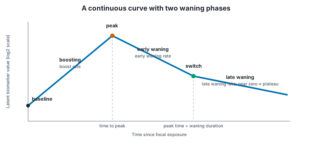
The kinetic parameterisation on the fitted log2 scale. Positive duration parameters enforce peak-before-switch ordering; a late waning rate near zero represents a long-term plateau.

Kinetic curve

For a participant-biomarker pair, let baseline be (b), time to peak (t_p), waning-rate change time (t_s > t_p), boost rate (r_b > 0), early waning rate (r_e > 0), and late waning rate (r_l > 0). The latent log2 mean is

$$\mu(t) = \begin{cases} b + r_b t, & t \le t_p, \\ b + r_b t_p - r_e(t-t_p), & t_p < t \le t_s, \\ b + r_b t_p - r_e(t_s-t_p) - r_l(t-t_s), & t > t_s. \end{cases}$$

The curve is continuous. The second post-peak rate is not structurally zero: it describes long-term waning, and a posterior near zero represents a plateau. This is the behaviour of the original Stan implementation and its defaults, despite older documentation calling the interval from tp to ts a plateau and saying m2 was fixed at zero. The clearer interpretation is boost, early waning, then late waning or plateau.

There is no artificial floor at zero on the model scale. The former max(mu, 0) caused a non-differentiable flat region and made the implied floor depend on a data-derived reference. With a fixed response transformation, log2 values below zero are valid positive response values below the reference.

Population, covariate, and participant effects

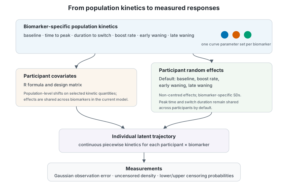
The default hierarchy from biomarker-specific population parameters to covariate-conditional and participant-specific trajectories. Peak timing and switch duration are shared across participants by default.

Each biomarker (k) has its own population baseline and five positive kinetic parameters. Let (q_k) be a positive population time or rate, (x_i) the participant design row, and (z_{q,i}(0,1)). Participant parameters are

$$b_{ik} = b_k + x_i^T\beta_b + \sigma_{b,k}z_{b,i}$$

and

$$q_{ik} = q_k\exp(x_i^T\beta_q + \sigma_{q,k}z_{q,i}).$$

Thus baseline effects are additive in log2 units, whereas positive time and rate effects are multiplicative. This guarantees positive rates, positive times, and (t_s > t_p) for every participant and covariate profile. The old additive construction could reverse rate signs or produce an individual change time before their peak.

Active random effects use a non-centred parameterisation. The standardised effect (z_{q,i}) is shared across biomarkers and scaled by a biomarker-specific standard deviation. This preserves an original scientific assumption: a participant high on a kinetic quantity for one biomarker tends to be high on that quantity for all biomarkers. A future model could estimate a richer cross-biomarker correlation structure, but this pass does not add it.

The default participant hierarchy includes baseline, boost_rate, early_waning_rate, and late_waning_rate. Participants may therefore differ in their baseline response, induction slope, and both waning components. Peak timing and waning_duration (the positive duration from peak to the switch in waning rate) have no residual participant random effect by default after conditioning on selected covariates. This is a modelling assumption supported by the motivating data and its posterior geometry, not a claim that transition timing can never vary biologically. Another dataset can opt into a different selected hierarchy or all six effects:

prepare_epikinetics_data(
  dat,
  participant_parameters = c(
    "baseline", "boost_rate", "early_waning_rate", "late_waning_rate"
  )
)

prepare_epikinetics_data(dat, participant_parameters = "all")

Inactive effects create neither latent standard-Normal parameters nor hierarchical SD parameters in Stan. Their reported participant SD is zero, and participant/new-participant predictions vary only over the fitted hierarchy.

Covariate coefficient vectors are also shared across biomarkers, preserving the original hierarchy. R constructs a conventional participant-level design matrix and records its contrasts so new profiles are encoded consistently. The default applies that matrix to every kinetic parameter, as the legacy model did, but the choice is no longer implicit. covariate_parameters can name a scientifically motivated subset:

prepare_epikinetics_data(
  dat,
  formula = ~ infection_history,
  covariate_parameters = c("baseline", "boost_rate", "late_waning_rate")
)

An active coefficient for baseline is an additive change in expected log2 level. For every positive time or rate it is a log ratio: exponentiating the coefficient gives the multiplicative population shift associated with a one-unit design-matrix change. Inactive parameter/formula combinations do not create unused Stan coefficients.

Priors

epikinetics_priors() defines one inspectable set of priors for population kinetics, participant and covariate scales, and observation error. Population priors are Normal; the five positive kinetic quantities are truncated at zero. Participant standard deviations and observation error have half-Normal priors, while regression coefficients have zero-centred Normal priors on their corresponding link scales.

set.seed(2026)
priors <- epikinetics::epikinetics_priors()
plot(priors, scale = "response", reference_value = 1)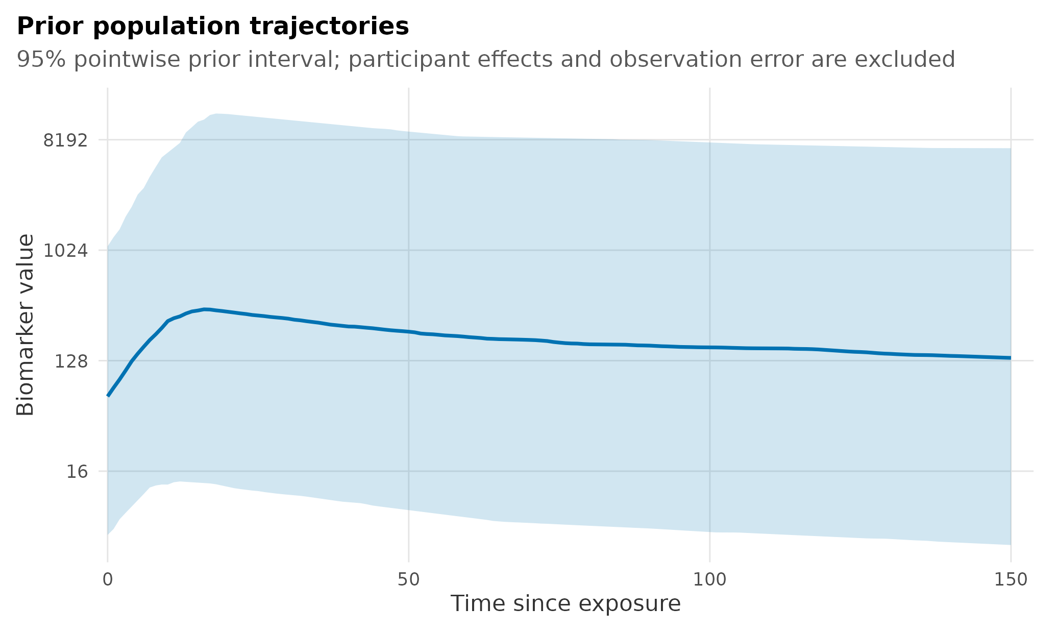

Latent population trajectories implied by the default kinetic-parameter priors. The median and 95% interval exclude participant variation and observation error so the population curve remains interpretable.

This is a prior check for the latent population curve, not a full predictive distribution for future measurements. Response-scale uncertainty is multiplicative, so the plot uses log2 spacing with natural response labels. Increasing ndraws stabilises estimated quantiles but does not narrow the prior.

Override only scientifically motivated quantities; unspecified fields retain their defaults:

priors <- epikinetics_priors(
  time_to_peak = c(mean = 12, sd = 4),
  early_waning_rate = c(mean = 0.025, sd = 0.01),
  observation_sd = 0.75
)

prepare_epikinetics_data(dat, priors = priors)

Stan transports standard-Normal raw variables through the configured truncated- or half-Normal inverse CDFs. This supplies the requested support and places default initial values on the scale of each prior; participant effects are non-centred separately through their standardised effects.

Observation and censoring model

For an uncensored measurement on the model scale,

$$y_n \sim \mathrm{Normal}(\mu_n,\sigma_{obs}).$$

The observation SD is common to biomarkers, as in the original model. A left-censored observation contributes normal_lcdf(lower_limit | mu, observation_sd) and a right-censored observation contributes normal_lcdf(mu | upper_limit, observation_sd). The latter is the exact Normal identity $\log P(Y \ge U)=\log \Phi((\mu-U)/\sigma)$, expressed in a numerically stable lower-tail form. It avoids a finite extreme upper-tail probability being rounded to log(0) during initialisation; it does not change the likelihood. Limits are row-level Stan vectors, so datasets may have no censoring, one-sided censoring, both sides, or biomarker/observation-specific limits without branching into separate models.

Computational implementation

Observations are sorted into contiguous participant ranges. Stan constructs participant-biomarker kinetics as local model-block values, rather than saving large transformed-parameter matrices in every posterior draw. reduce_sum partitions the likelihood by participant, preserving locality and amortising the participant-level parameter construction over each participant’s observations. The model is always compiled with STAN_THREADS; users control parallel chains with parallel_chains and within-chain workers with threads_per_chain.

Only the population waning change time is retained as a transformed parameter. Participant quantities and derived response-scale summaries are reconstructed from compact posterior draws in R.

The source is installed at stan/epikinetics.stan and is deliberately direct: one curve function, one participant-partitioned likelihood function, and the hierarchical model.

Every selected participant hierarchy is non-centred. The bundled example has a median of six observations per participant (some have only three), so a centred parameterisation would reintroduce the usual group-scale funnel. The more consequential geometry problem was not centred versus non-centred: it was asking sparse participant series to identify all six random kinetic effects. The explicit participant_parameters selection avoids that overfitting while leaving the full model available when study design and diagnostics support it.

For the practical workflow, return to Getting started; the Covariates and Censoring articles give shorter introductions to those parts of the hierarchy.