Getting started with epikinetics

epikinetics fits hierarchical kinetics models to repeated positive biomarker measurements after one focal exposure. This page is the shortest path from a data frame to a fitted population trajectory; the focused articles linked at the end explain each step.

Prepare the data

The package bundles public neutralising-antibody data for examples. Preparation is deliberately separate from fitting, so every transformation can be checked before starting Stan.

library(epikinetics)

dat <- read.csv(
  system.file("extdata", "delta.csv", package = "epikinetics")
)

prepared <- prepare_epikinetics_data(
  dat,
  formula = ~ infection_history,
  biomarker_order = c("Ancestral", "Alpha", "Delta"),
  lower_limit = 5,
  upper_limit = 2560
)

prepared

#> Prepared epikinetics model data
#>   Observations: 2255
#>   Participants: 335
#>   Biomarkers:   3 (Ancestral, Alpha, Delta; explicit order)
#>   Covariates:   infection_history
#>   Effects on:  baseline, time_to_peak, waning_duration, boost_rate, early_waning_rate, late_waning_rate
#>   Random effects: baseline, boost_rate, early_waning_rate, late_waning_rate
#>   Censoring:    none=2003, left=126, right=126
#>   Time range:     0 to 578 since exposure
#>   Model scale:  log2(value / 1); range  2.321928 to 11.321928
#>   Exposure:     one fixed focal exposure per participant

prediction_grid(prepared)

#>   .profile                 infection_history
#> 1        1                   Infection naive
#> 2        2 Previously infected (Pre-Omicron)

Use summary(prepared), model.matrix(prepared), and stan_data(prepared) to inspect the validated observations, formula encoding, participant/biomarker indices, censoring limits, and exact Stan data. The Data, Covariates, and Censoring articles describe those contracts.

Fit and diagnose

CmdStan is installed explicitly once with cmdstanr::install_cmdstan(). The first fit compiles and caches the threaded model; later fits reuse it.

fit <- fit_epikinetics(
  prepared,
  chains = 4,
  parallel_chains = 4,
  threads_per_chain = 2,
  seed = 2026
)

fit
diagnose_epikinetics(fit)

Do not interpret posterior estimates until the diagnostic summary is satisfactory. Fitting the model explains the computational arguments, and Diagnostics explains the checks.

Predict population kinetics

pred <- predict(fit, type = "population", times = 0:150)
plot(pred)

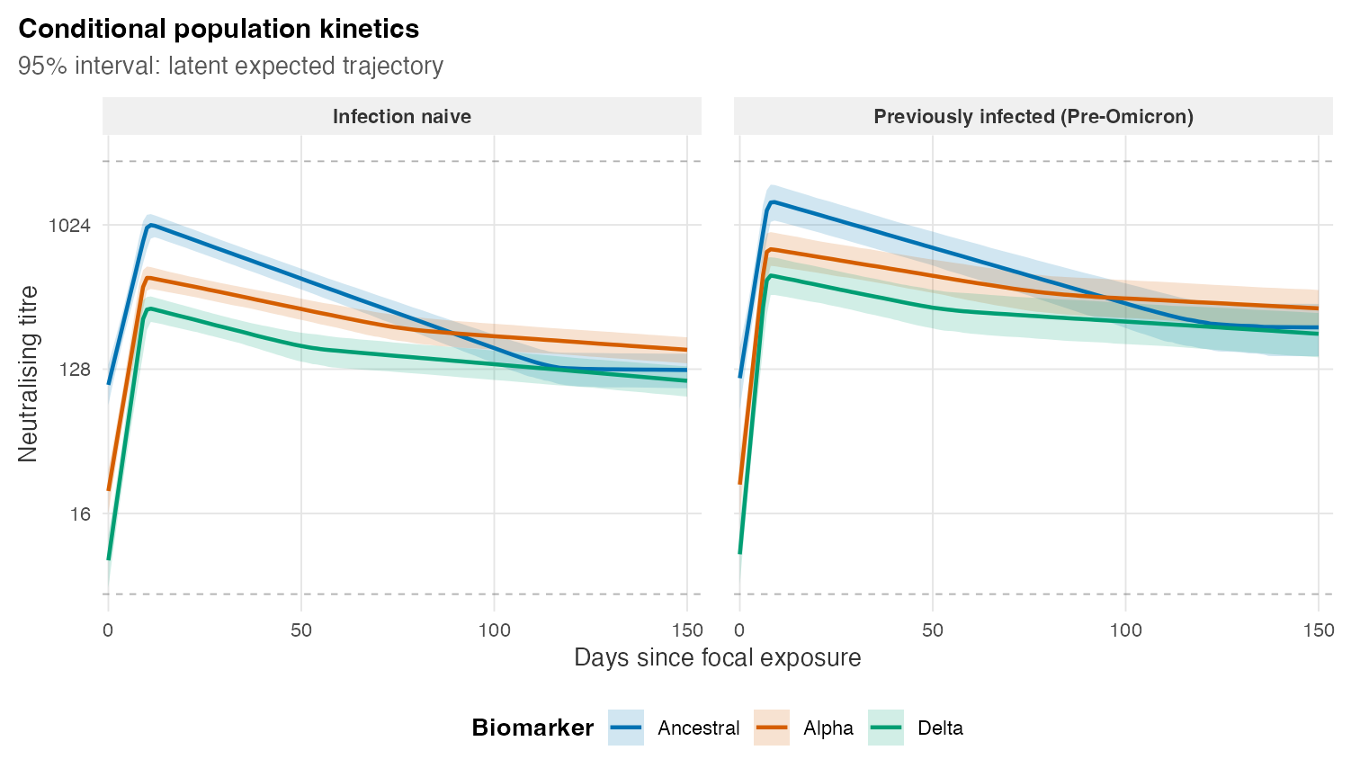
Conditional population kinetics produced by the code above. Biomarkers are overlaid by colour; infection-history profiles define panels. Lines are posterior medians and ribbons are 95% credible intervals for the latent trajectories.

The figure is precomputed from an actual four-chain package fit so routine documentation builds do not rerun MCMC. Both posterior mean and median remain in pred; the plotting method uses the median by default.

Continue with Population-level kinetics for prediction grids, newdata, and uncertainty targets, or Individual-level kinetics to reconstruct fitted participants. The case study then combines the workflow in a complete applied analysis.