Case Study 1: Simulation Recovery

R Code Description

This document describes the steps and components of the provided R code for creating and running serological models using simulated data. The code defines observational models, antibody kinetics models, and runs inference using MCMC methods.

Step 1: Load Required Libraries

library(devtools)
library(tidyr)
library(dplyr)
library(magrittr)
library(serojump)
#devtools::load_all()
library(patchwork)

# Using more than one core might fail on windows, 
if (.Platform$OS.type == "windows") {
  mc.cores <- 1
} else {
  mc.cores <- 2 # use as many as available, preferably 4.
}

Step 2: Read Simulated Data

This data has been generated using serosim. The code the generate this data can be found at in the folder serosim in the package repo. The data is generated using the cesCOP and cesNoCOP models.

sim_model_cop <- readRDS(file = "cesCOP_inputs.RDS")
sim_res_cop <- readRDS(file = "cesCOP_sim_data_0.5.rds")

#sim_model_cop <- readRDS(file = system.file("extdata", "vig_data", "cesCOP", "cesCOP_inputs.RDS", package = "serojump"))
#sim_res_cop <- readRDS(file = system.file("extdata","vig_data", "cesCOP", "cesCOP_sim_data_0.5.RDS", package = "serojump"))

#modeli <- readRDS(file = "cesCOP_inputs.RDS")
#modeli <- readRDS(file = "cesCOP_sin_data_0.5.RDS")

data_titre_model <- sim_res_cop$observed_biomarker_states %>% select(i, t, value) %>% rename(id = i, time = t, titre = value) 
data_titre_model <- data_titre_model %>% mutate(biomarker = "sVNT") %>% as.data.frame %>% rename(sVNT = titre)

# Check the entries are sensible
check_sero_no_single_entries(data_titre_model)

## No single entries in data_sero!,

check_sero_timings(data_titre_model)

## No individuals with less than 15 days in the study!

Step 3: Define Likelihood and Kinetics Functions

obsLogLikelihood <- function(titre_val, titre_est, pars) {
    ll <- dnorm(titre_val, titre_est, pars[1], log = TRUE)
}

infSerumKinetics <- function(titre_est, timeSince, pars) {
    a <- pars[1]
    b <- pars[2]
    c <- pars[3]
    if (timeSince < 14) {
        titre_est <- titre_est + log(exp(a) + exp(c)) * (timeSince) / 14;
    } else {
        titre_est <- titre_est + log(exp(a) * exp(-b/10 * (timeSince - 14)) + exp(c));
    }
    titre_est
}

noInfSerumKinetics <- function(titre_est, timeSince, pars) {
    titre_est_log <- titre_est - pars[1] * (timeSince)
    titre_est_log <- max(0, titre_est_log)
    titre_est_log
}

Step 4: Define the Observational and Kinetics Models

# Define the biomarkers and exposure types in the model
biomarkers <- c("sVNT")
exposureTypes <- c("none", "inf")
exposureFitted <- "inf"

# Define the observational model
observationalModel <- list(
    names = c("sVNT"),
    model = makeModel(
        addObservationalModel("sVNT", c("sigma"), obsLogLikelihood)
        ), # observational model,
    prior = bind_rows(
            addPrior("sigma", 0.0001, 4, "unif", 0.0001, 4)
    )
)

# Define the antibody kinetics model
abkineticsModel <- list(
    model = makeModel(
            addAbkineticsModel("none", "sVNT", "none",  c("wane"), noInfSerumKinetics),
            addAbkineticsModel("inf", "sVNT", "inf", c("a", "b", "c"), infSerumKinetics)
        ),
    prior = bind_rows(
        addPrior("wane", 0.0, 0.01, "unif", 0.0, 0.01), # observational model
        addPrior("a", -6, 6, "norm",  2, 2), # ab kinetics
        addPrior("b", 0, 1, "norm",  0.3, 0.05), # ab kinetics
        addPrior("c", 0, 4, "unif", 0,  4) # ab kinetics 
    )
)



model_cop <- createSeroJumpModel(
    data_sero = data_titre_model, 
    data_known = NULL,
    biomarkers = biomarkers,
    exposureTypes = exposureTypes,
    exposureFitted = exposureFitted,
    observationalModel = observationalModel,
    abkineticsModel = abkineticsModel)

## OUTLINE OF INPUTTED MODEL
## There are  1  measured biomarkers:  sVNT 
## There are  2  exposure types in the study period:  none, inf 
## The fitted exposure type is  inf 
## PRIOR DISTRIBUTIONS 
## Prior parameters of observationalModel are:  sigma 
## Prior parameters of abkineticsModel are:  wane, a, b, c 
## No single entries in data_sero!, 
## No individuals with less than 15 days in the study! 
## Exposure rate is not defined over the time period. Defaulting to uniform distribution between 1 and  119 .

Step 4B: Prerun sanity plots

Before running the whole model it is good to check the data and the priors. This can be done using a suit of functions plotPriors function.

p1 <- plotSero(model_cop)
p2 <- plotPriorPredictive(model_cop)

## Warning: Using `size` aesthetic for lines was deprecated in ggplot2 3.4.0.
## ℹ Please use `linewidth` instead.
## ℹ The deprecated feature was likely used in the serojump package.
##   Please report the issue to the authors.
## This warning is displayed once per session.
## Call `lifecycle::last_lifecycle_warnings()` to see where this warning was
## generated.

p3 <- plotPriorInfection(model_cop)
p1 / p2

## Ignoring unknown labels:
## • colour : "Exposure type"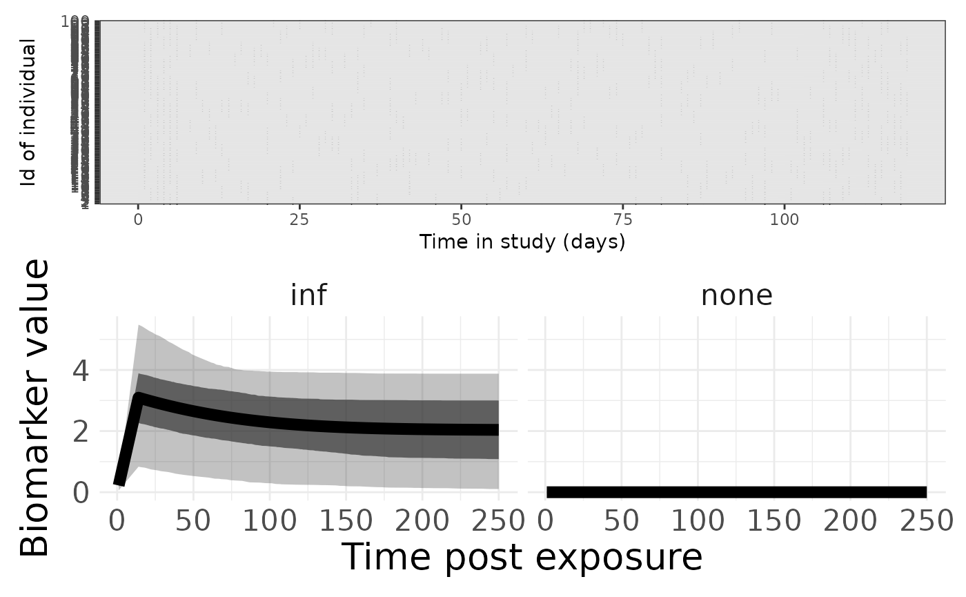

p3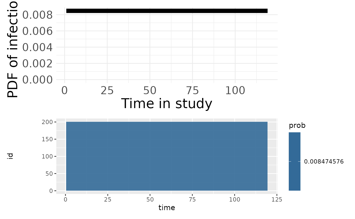

Step 5: Define the Complete Model

sim_model_no_cop <- readRDS(file = "cesNoCOP_inputs.RDS")
sim_res_no_cop <- readRDS(file = "cesNoCOP_sim_data_0.5.rds")

#modeli <- readRDS(file = system.file("extdata", "vig_data", "cesNoCOP", "cesNoCOP_inputs.RDS", package = "serojump"))
#res <- readRDS(file = system.file("extdata", "vig_data", "cesNoCOP", "cesNoCOP_sim_data_0.5.RDS", package = "serojump"))

data_titre_model <- sim_res_no_cop$observed_biomarker_states %>% select(i, t, value) %>% rename(id = i, time = t, titre = value) 
data_titre_model <- data_titre_model %>% mutate(biomarker = "sVNT") %>% as.data.frame %>% rename(sVNT = titre)


model_no_cop <- createSeroJumpModel(
    data_sero = data_titre_model, 
    data_known = NULL,
    biomarkers = biomarkers,
    exposureTypes = exposureTypes,
    exposureFitted = exposureFitted,
    observationalModel = observationalModel,
    abkineticsModel = abkineticsModel)

## OUTLINE OF INPUTTED MODEL
## There are  1  measured biomarkers:  sVNT 
## There are  2  exposure types in the study period:  none, inf 
## The fitted exposure type is  inf 
## PRIOR DISTRIBUTIONS 
## Prior parameters of observationalModel are:  sigma 
## Prior parameters of abkineticsModel are:  wane, a, b, c 
## No single entries in data_sero!, 
## No individuals with less than 15 days in the study! 
## Exposure rate is not defined over the time period. Defaulting to uniform distribution between 1 and  119 .

Step 5B: Prerun sanity plots