Multidimensional Correlates of Protection with seroCOP • seroCOP

Joint Biomarker CoP

SeroMulti fits one joint model to 2–4 antibody biomarkers measured for the same person and time point. Each biomarker has its own EC50 and positive slope. For $D$ biomarkers, the joint signal is

$\eta = \sum_{d=1}^{D} \text{slope}_d (\text{titre}_d - \text{ec50}_d).$

The CoP rises when the combined biomarker signal increases. This vignette uses two biomarkers, so the fitted CoP can be inspected as a surface. Three- and four-biomarker models use the same interface, but are evaluated at chosen biomarker combinations rather than drawn as a surface.

library(seroCOP)
library(ggplot2)
set.seed(2026)

Simulate a Two-Biomarker Study

n <- 300
titres <- cbind(
  IgG = rnorm(n, mean = 2.2, sd = 1.0),
  Neutralisation = rnorm(n, mean = 1.8, sd = 0.9)
)

true_floor <- 0.05
true_ceiling <- 0.75
true_ec50 <- c(IgG = 2.0, Neutralisation = 1.5)
true_slope <- c(IgG = 1.1, Neutralisation = 0.9)
eta <- as.vector((titres - rep(true_ec50, each = n)) %*% true_slope)
infection_probability <- true_ceiling *
  (plogis(-eta) * (1 - true_floor) + true_floor)
infected <- rbinom(n, size = 1, prob = infection_probability)

head(data.frame(titres, infected))
#>         IgG Neutralisation infected
#> 1  2.720589       1.666267        1
#> 2  1.120309       1.635343        1
#> 3  2.339238       1.027667        0
#> 4  2.115251       2.662343        0
#> 5  1.533360       1.044831        1
#> 6 -0.316089       1.116248        0

Visualise the Joint CoP Surface

The simulation gives a known surface before fitting. It provides a visual reference for the fitted posterior surface below.

surface_grid <- expand.grid(
  IgG = seq(min(titres[, "IgG"]), max(titres[, "IgG"]), length.out = 80),
  Neutralisation = seq(min(titres[, "Neutralisation"]),
                       max(titres[, "Neutralisation"]), length.out = 80)
)
grid_eta <- as.vector((as.matrix(surface_grid) -
  rep(true_ec50, each = nrow(surface_grid))) %*% true_slope)
grid_risk <- true_ceiling * (plogis(-grid_eta) * (1 - true_floor) + true_floor)
surface_grid$cop <- 1 - grid_risk / true_ceiling

ggplot(surface_grid, aes(x = IgG, y = Neutralisation, fill = cop)) +
  geom_raster(interpolate = TRUE) +
  geom_contour(aes(z = cop), color = "white") +
  scale_fill_viridis_c(name = "CoP") +
  labs(title = "Simulated joint correlate-of-protection surface") +
  theme_minimal()
#> Warning: The following aesthetics were dropped during statistical transformation: fill.
#> ℹ This can happen when ggplot fails to infer the correct grouping structure in
#>   the data.
#> ℹ Did you forget to specify a `group` aesthetic or to convert a numerical
#>   variable into a factor?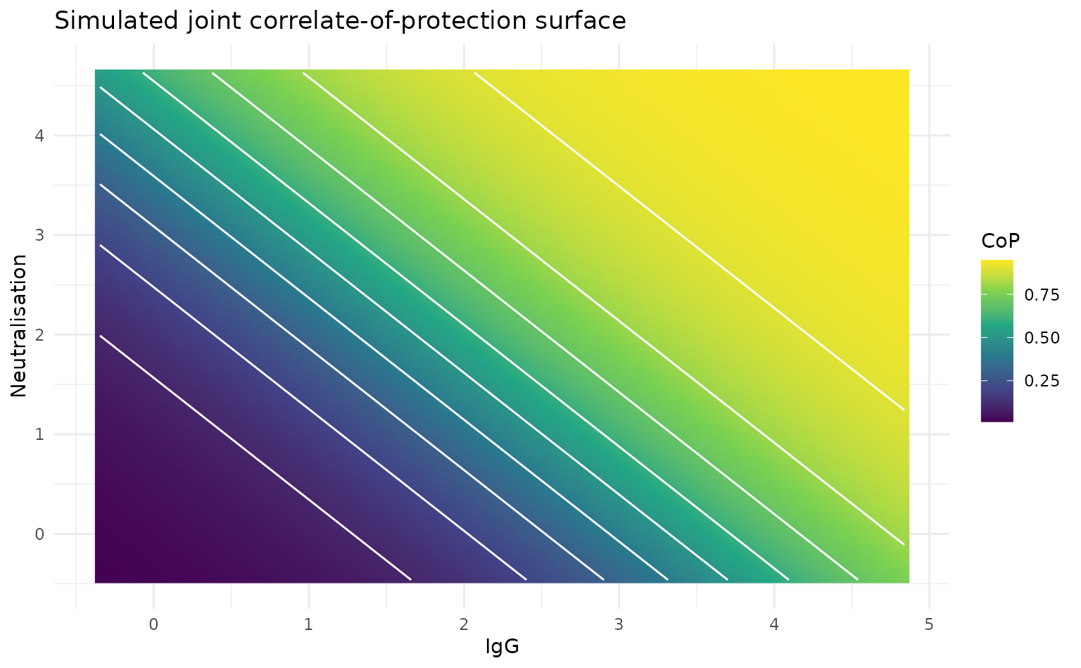

Fit SeroMulti

model <- SeroMulti$new(titre = titres, infected = infected)
model$fit_model(chains = 4, iter = 2000, warmup = 1000, cores = 4)

Plot the Fitted Surface

After fitting, plot_surface() summarises posterior CoP draws across a grid. It returns a ggplot filled-contour plot by default; type = "persp" draws a base-R perspective surface.

model$plot_surface(type = "contour")
model$plot_surface(type = "persp")

Three and Four Biomarkers

For higher-dimensional models, supply a 3- or 4-column matrix. Posterior CoP values can then be obtained for observed or selected biomarker combinations.

three_marker_titres <- cbind(titres, IgA = rnorm(n, 1.6, 0.8))
three_marker_model <- SeroMulti$new(three_marker_titres, infected)
three_marker_model$fit_model(chains = 4, iter = 2000, warmup = 1000, cores = 4)

posterior_cop <- three_marker_model$predict_protection(three_marker_titres)
colMeans(posterior_cop)