Hierarchical Group Effects in seroCOP
Source:vignettes/hierarchical-groups.Rmd
hierarchical-groups.RmdIntroduction
This vignette demonstrates how to use hierarchical modeling in
SeroCOP to account for group-level heterogeneity in
correlates of protection. This is particularly useful when different
subpopulations (e.g. age groups, geographic regions, or vaccine types)
may have different dose–response relationships.
When to Use Hierarchical Models
Hierarchical modeling is appropriate when:
- You have multiple groups that may differ in their correlate of protection relationships
- You want to “borrow strength” across groups while allowing group-specific estimates
- Sample sizes within groups may be modest
- You want to quantify between-group variability in protection
Example Scenario: Age-Specific Correlates
We demonstrate with a realistic scenario where the strength of the antibody–protection relationship varies by age group:
- Young adults (largest cohort): Steep relationship — strong correlate
- Middle-aged (medium cohort): Moderate relationship
- Older adults (smallest cohort): Flat — weak or absent correlate
Simulate Age-Stratified Data
The three age groups have different sample sizes to reflect typical epidemiological studies where recruitment is unequal.
# ---- unequal group sizes ----
young_n  <- 150   # most participants
middle_n <- 90
old_n    <- 45    # fewest participants

simulate_group <- function(n, group_name, slope, ec50,
                           floor = 0.05, ceiling = 0.70) {
  titre <- rnorm(n, mean = 2.5, sd = 2.0)
  logit_part     <- 1 / (1 + exp(slope * (titre - ec50)))
  prob_infection <- ceiling * (logit_part * (1 - floor) + floor)
  infected       <- rbinom(n, 1, prob_infection)
  data.frame(titre = titre, infected = infected, age_group = group_name)
}

young  <- simulate_group(young_n,  "Young adults",   slope = 3.0, ec50 = 1.5)
middle <- simulate_group(middle_n, "Middle-aged",    slope = 1.5, ec50 = 1.8)
old    <- simulate_group(old_n,    "Older adults",   slope = 0.3, ec50 = 2.0)

all_data <- rbind(young, middle, old)
# Use an ordered factor so panels appear in a natural left-to-right order
all_data$age_group <- factor(all_data$age_group,
                             levels = c("Young adults", "Middle-aged", "Older adults"))

cat("Simulated data with age-specific correlates:\n")
#> Simulated data with age-specific correlates:
cat(sprintf("  Young adults  (n=%d): slope=3.0, ec50=1.5 — strong correlate\n", young_n))
#>   Young adults  (n=150): slope=3.0, ec50=1.5 — strong correlate
cat(sprintf("  Middle-aged   (n=%d): slope=1.5, ec50=1.8 — moderate correlate\n", middle_n))
#>   Middle-aged   (n=90): slope=1.5, ec50=1.8 — moderate correlate
cat(sprintf("  Older adults  (n=%d): slope=0.3, ec50=2.0 — weak correlate\n", old_n))
#>   Older adults  (n=45): slope=0.3, ec50=2.0 — weak correlate
cat(sprintf("\nTotal n=%d  |  Infection rate: %.1f%%\n",
            nrow(all_data), 100 * mean(all_data$infected)))
#>
#> Total n=285  |  Infection rate: 28.1%
Raw Data: Binned Infection Rates
Before fitting, it is helpful to summarise the raw data by binning titres and computing the observed infection proportion in each bin. These empirical points will later be overlaid on the fitted curves to assess goodness-of-fit.
# Bin titre into deciles *within each age group*
n_bins <- 8

all_data$bin <- ave(
  all_data$titre, all_data$age_group,
  FUN = function(x) {
    breaks <- unique(quantile(x, probs = seq(0, 1, length.out = n_bins + 1)))
    as.integer(cut(x, breaks = breaks, include.lowest = TRUE))
  }
)

# Summarise per group × bin
binned <- aggregate(
  cbind(infected, titre) ~ age_group + bin,
  data    = all_data,
  FUN     = mean
)
bin_n <- aggregate(infected ~ age_group + bin, data = all_data, FUN = length)
binned$n <- bin_n$infected

head(binned)
#>      age_group bin  infected      titre  n
#> 1 Young adults   1 0.6842105 -0.5614768 19
#> 2  Middle-aged   1 0.5000000 -0.3363742 12
#> 3 Older adults   1 0.6666667 -0.2649755  6
#> 4 Young adults   2 0.7894737  0.6731679 19
#> 5  Middle-aged   2 0.4545455  0.7761623 11
#> 6 Older adults   2 0.1666667  0.6798197  6
ggplot(binned, aes(x = titre, y = infected, colour = age_group)) +
  geom_point(aes(size = n), alpha = 0.7) +
  geom_line(aes(group = age_group), alpha = 0.5, linetype = "dashed") +
  scale_size_area(max_size = 8, guide = guide_legend(title = "Bin n")) +
  facet_wrap(~age_group) +
  labs(
    title    = "Raw Binned Infection Rates by Age Group",
    x        = "Mean Titre in Bin (log scale)",
    y        = "Observed Infection Proportion",
    colour   = "Age Group"
  ) +
  theme_minimal() +
  theme(legend.position = "bottom", plot.title = element_text(hjust = 0.5, face = "bold"))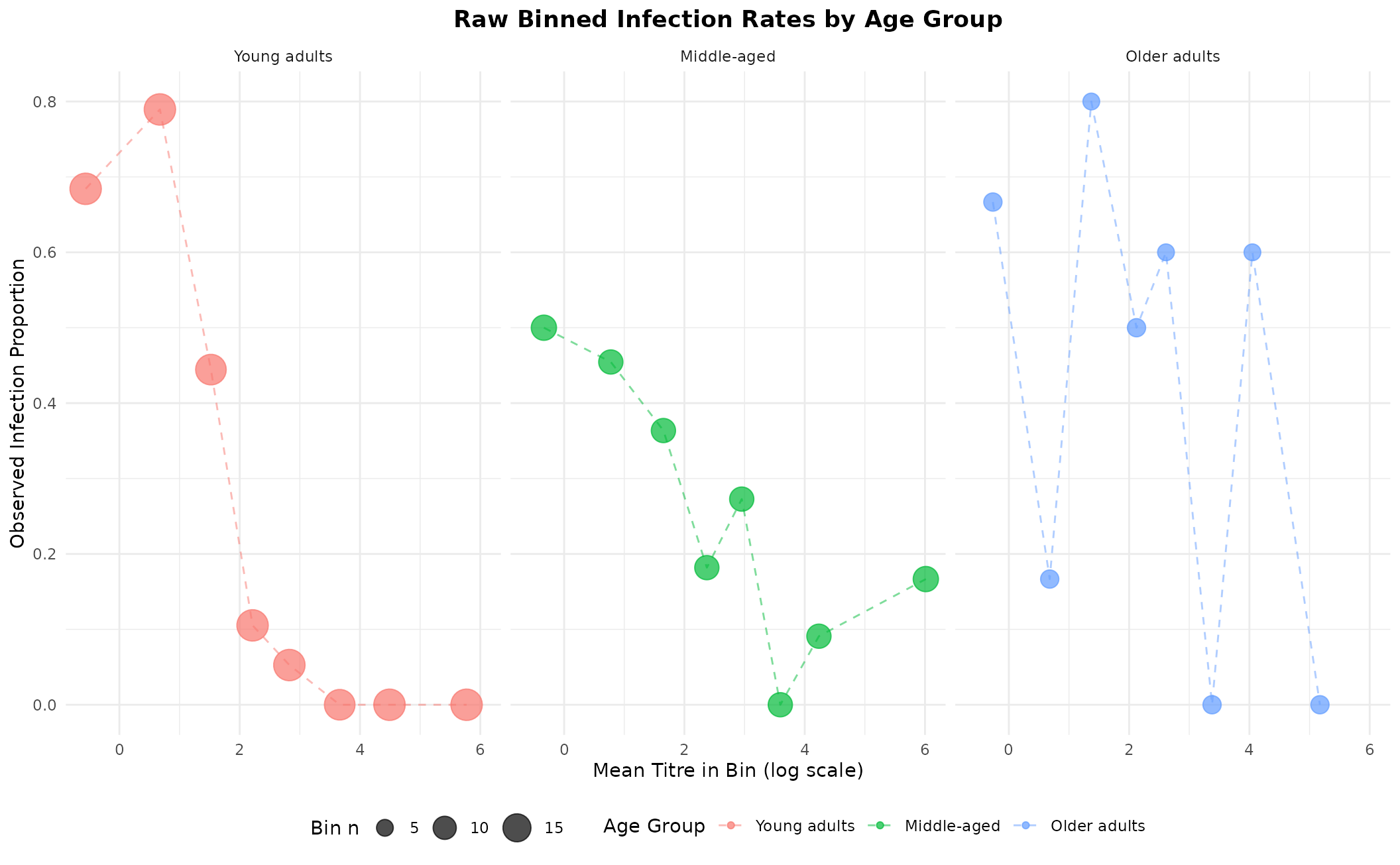
Binned observed infection rates (point area ∝ bin size). These will be overlaid on fitted curves later.
Fit the Hierarchical Model
The hierarchical model estimates group-specific ec50 and
slope values while sharing a common floor and
ceiling. Group-level random effects borrow strength across
age groups.
By default, ceiling is fixed across groups (shared
attack rate). Pass ceiling_group = TRUE if you expect the
baseline attack rate to differ by group.
hier_model <- SeroCOP$new(
  titre    = all_data$titre,
  infected = all_data$infected,
  group    = all_data$age_group
)

hier_model$fit_model(
  chains        = 4,
  iter          = 2000,
  warmup        = 1000,
  cores         = 1,
  ceiling_group = FALSE,   # shared ceiling (default)
  refresh       = 0
)
Fitted Curves with Binned Data Overlay
The plot below shows the posterior mean curve and 95% credible interval for each age group, with the marginalised (population-weighted) curve as a dashed black line. Empirical binned points are overlaid to allow visual assessment of model fit.
# --- 1. Get fitted curve data via the built-in method -------------------------
p_base <- hier_model$plot_group_curves(
  title       = "Age-Specific Correlates of Risk with Empirical Bins",
  weights_pop = c("Young adults"  = young_n,
                  "Middle-aged"   = middle_n,
                  "Older adults"  = old_n)
)

# --- 2. Overlay binned empirical points (size ∝ bin n) -----------------------
p_base +
  geom_point(
    data    = binned,
    mapping = aes(x = titre, y = infected, size = n),
    colour  = "black", alpha = 0.75, inherit.aes = FALSE
  ) +
  scale_size_area(max_size = 7, guide = guide_legend(title = "Bin n")) +
  theme(legend.position = "bottom")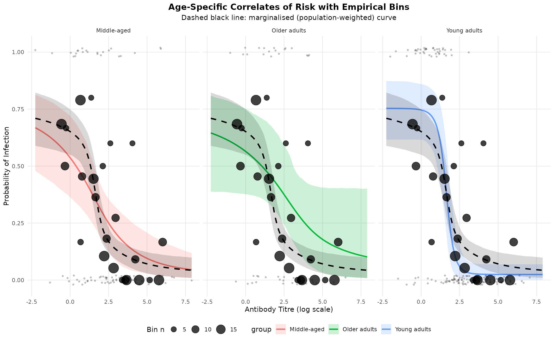
The black dots are the raw binned proportions. When they track the fitted curve closely, it indicates a good fit. Deviations suggest model mis-specification or sparse data in that titre region.
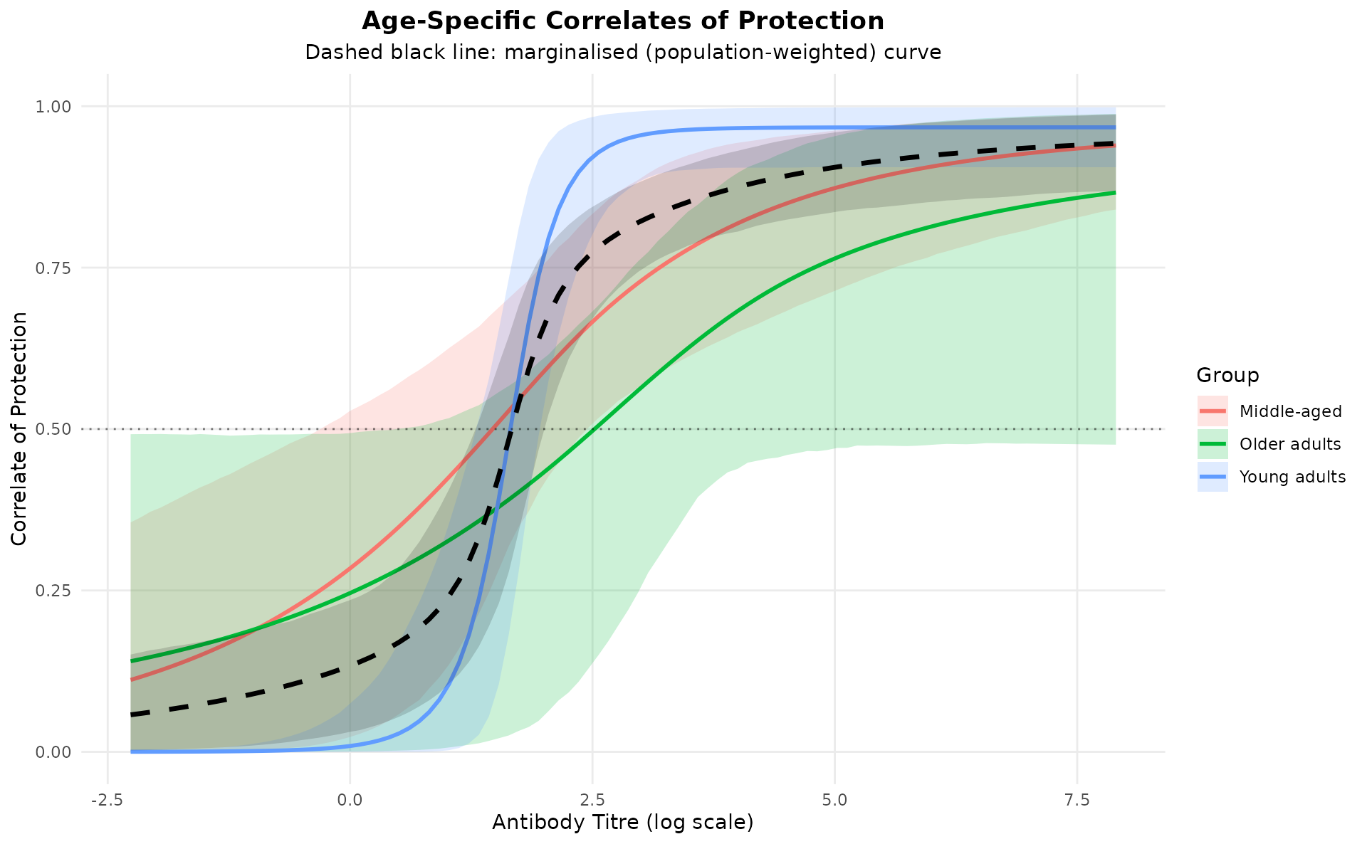
Correlates of Protection Curves
The correlate of protection (COP) is defined as:
This quantifies the probability of being protected conditional on exposure. The population-weighted marginalised COP curve summarises the overall effectiveness across age groups.
hier_model$plot_cop_curves(
  title       = "Age-Specific Correlates of Protection",
  weights_pop = c("Young adults"  = young_n,
                  "Middle-aged"   = middle_n,
                  "Older adults"  = old_n)
)
Extract Group-Specific Parameters
group_params <- hier_model$extract_group_parameters()
print(group_params)
#>          group parameter      mean    median         sd         q025      q975
#> 1 Young adults   ceiling 0.7535608 0.7562615 0.06530828  0.616718632 0.8736953
#> 2 Young adults      ec50 1.6228170 1.6269624 0.16381614  1.273193288 1.9407667
#> 3 Young adults     slope 4.2703235 3.9450179 1.76451069  1.802135171 8.6867585
#> 4  Middle-aged   ceiling 0.7535608 0.7562615 0.06530828  0.616718632 0.8736953
#> 5  Middle-aged      ec50 1.2456847 1.3545520 0.68539125 -0.438686108 2.3425992
#> 6  Middle-aged     slope 0.7637980 0.6446116 0.51850845  0.259426276 2.0535662
#> 7 Older adults   ceiling 0.7535608 0.7562615 0.06530828  0.616718632 0.8736953
#> 8 Older adults      ec50 2.1579099 2.0386108 0.95894496  0.453728701 4.1092192
#> 9 Older adults     slope 0.6560202 0.5138150 0.60495916 -0.004831226 2.3138291
Key observations:
-
Young adults have the steepest
slope— a strong antibody correlate -
Older adults have a
slopenear zero — little titre-dependent protection - Middle-aged are intermediate
-
ec50shifts to the right with age — older individuals need higher titres for equivalent protection
Model Performance
Overall and Per-Group Metrics
metrics <- hier_model$get_metrics()
#> Performance Metrics:
#>   ROC AUC (marginalised):        0.807
#>   ROC AUC (within-group wtd):    0.812
#>   Brier Score:                   0.136
#>   LOO ELPD:                      -125.64 (SE: 9.03)
#>   LOO ELPD by group:
#>     Young adults           -46.12 (SE: 6.30, n = 150)
#>     Middle-aged            -49.23 (SE: 5.45, n = 90)
#>     Older adults           -30.29 (SE: 2.53, n = 45)
The per-group LOO-ELPD breakdown shows how much each age group contributes to (or detracts from) overall model fit. A lower ELPD for a group indicates the model fits that group less well — often because it has fewer participants or a weaker signal.
Comparison with Pooled Model
pooled_model <- SeroCOP$new(
  titre    = all_data$titre,
  infected = all_data$infected
)

pooled_model$fit_model(
  chains  = 4,
  iter    = 2000,
  warmup  = 1000,
  cores   = 1,
  refresh = 0
)
hier_loo   <- hier_model$loo$estimates["elpd_loo", c("Estimate", "SE")]
pooled_loo <- pooled_model$loo$estimates["elpd_loo", c("Estimate", "SE")]

loo_diff <- hier_loo["Estimate"] - pooled_loo["Estimate"]
loo_se   <- sqrt(hier_loo["SE"]^2 + pooled_loo["SE"]^2)

cat("=== Model Comparison (LOO-CV) ===\n")
#> === Model Comparison (LOO-CV) ===
cat(sprintf("Hierarchical ELPD: %.2f (SE: %.2f)\n", hier_loo["Estimate"],   hier_loo["SE"]))
#> Hierarchical ELPD: -125.64 (SE: 9.03)
cat(sprintf("Pooled       ELPD: %.2f (SE: %.2f)\n", pooled_loo["Estimate"], pooled_loo["SE"]))
#> Pooled       ELPD: -134.95 (SE: 9.45)
cat(sprintf("Difference:        %.2f (SE: %.2f)  |  Z = %.2f\n",
            loo_diff, loo_se, loo_diff / loo_se))
#> Difference:        9.31 (SE: 13.07)  |  Z = 0.71

if (loo_diff > 2 * loo_se) {
  cat("-> Strong evidence favouring hierarchical model\n")
} else if (loo_diff > 0) {
  cat("-> Hierarchical preferred but evidence is weak\n")
} else {
  cat("-> No clear advantage for hierarchical model\n")
}
#> -> Hierarchical preferred but evidence is weak
Fitted Curves: Pooled Model vs Binned Data
The pooled model uses a single curve for all age groups. Overlaying the binned empirical rates highlights how much signal is lost by ignoring heterogeneity.
titre_grid  <- seq(min(all_data$titre), max(all_data$titre), length.out = 100)
pooled_pred <- pooled_model$predict(newdata = titre_grid)

pooled_df <- data.frame(
  titre = titre_grid,
  prob  = colMeans(pooled_pred),
  lower = apply(pooled_pred, 2, quantile, probs = 0.025),
  upper = apply(pooled_pred, 2, quantile, probs = 0.975)
)

ggplot() +
  geom_ribbon(data = pooled_df,
              aes(x = titre, ymin = lower, ymax = upper),
              fill = "gray70", alpha = 0.4) +
  geom_line(data = pooled_df,
            aes(x = titre, y = prob),
            colour = "gray30", linewidth = 1.2) +
  geom_point(data    = binned,
             mapping = aes(x = titre, y = infected,
                           colour = age_group, size = n),
             alpha = 0.85) +
  scale_size_area(max_size = 7, guide = guide_legend(title = "Bin n")) +
  facet_wrap(~age_group) +
  labs(
    title    = "Pooled Model vs Binned Empirical Rates",
    subtitle = "Gray band = pooled model; coloured points = within-group empirical proportions",
    x        = "Antibody Titre (log scale)",
    y        = "Probability of Infection",
    colour   = "Age Group"
  ) +
  theme_minimal() +
  theme(legend.position = "bottom",
        plot.title = element_text(hjust = 0.5, face = "bold"),
        plot.subtitle = element_text(hjust = 0.5))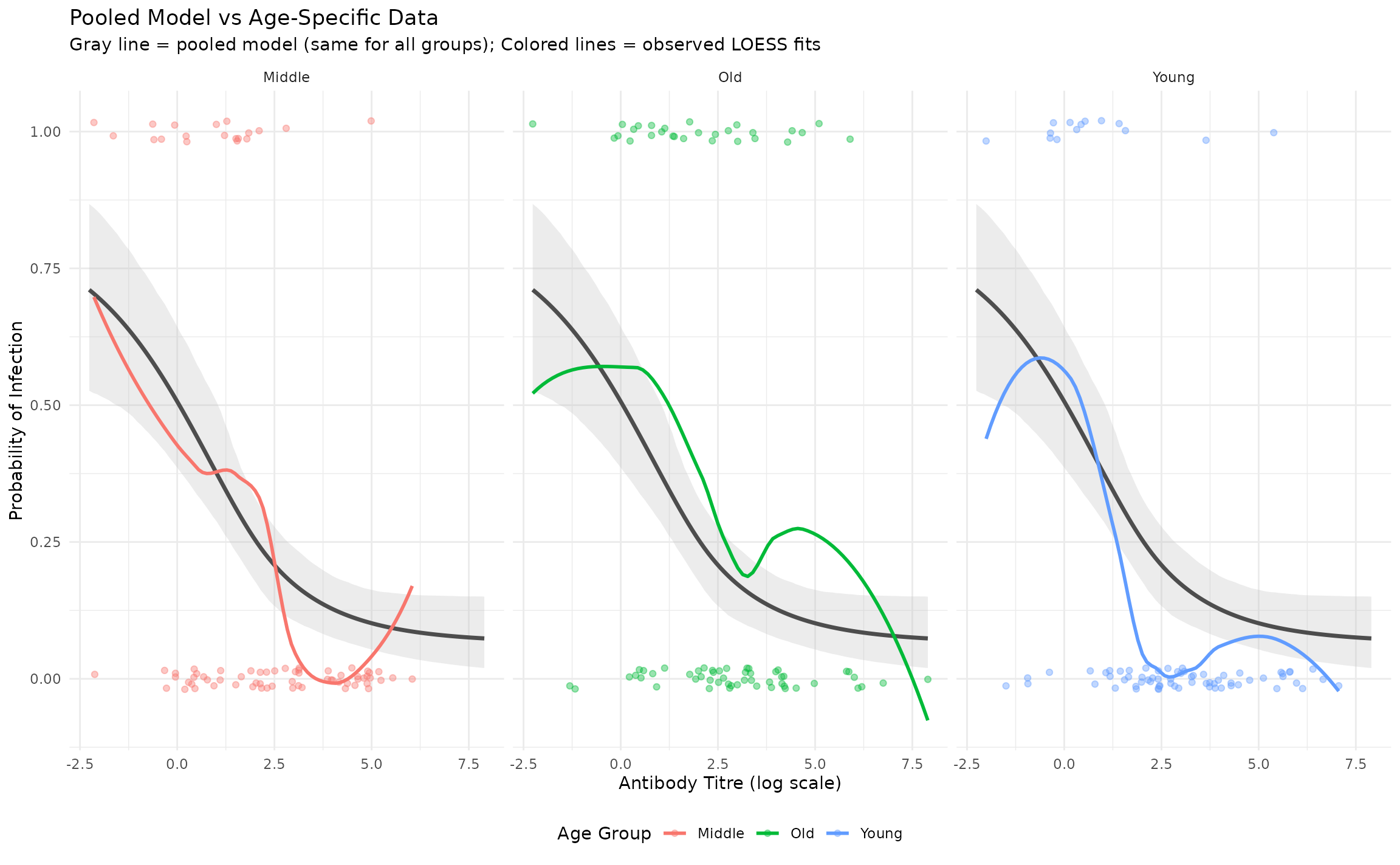
Technical Details
Model Structure
The hierarchical model uses random intercepts on ec50
and slope:
infected ~ ceiling * (inv_logit(-slope * (titre - ec50)) * (1 - floor) + floor)
floor    ~ 1
ceiling  ~ 1                   # fixed across groups (ceiling_group = FALSE)
ec50     ~ 1 + (1 | group)     # random intercept per group
slope    ~ 1 + (1 | group)     # random intercept per group
Set ceiling_group = TRUE in fit_model() to
also allow the ceiling (maximum attack rate) to vary across groups.
Priors
- Group-level standard deviations:
student_t(3, 0, 2.5)— weakly informative, permitting substantial between-group variation while regularising extremes. - Population-level: Beta priors on
floor/ceiling; Normal onec50(centred on data midpoint) andslope.
Population Weights for Marginalisation
Pass a named numeric vector to weights_pop in
plot_group_curves() and plot_cop_curves() to
control how the marginalised curve is computed:
# Census-based age-group proportions (must sum to any positive value)
hier_model$plot_cop_curves(
  weights_pop = c("Young adults" = 0.45, "Middle-aged" = 0.35, "Older adults" = 0.20)
)
If weights_pop = NULL (default), sample proportions are
used instead.
Conclusion
SeroCOP hierarchical models provide a flexible framework
for analysing correlates of protection with group-level
heterogeneity:
- Group-specific
ec50andslopeare estimated while borrowing strength - The shared
ceilingensures identifiability;ceiling_group = TRUErelaxes this - Binned empirical overlays give a quick visual goodness-of-fit check
- Per-group LOO contributions identify groups driving poor fit
-
plot_cop_curves()summarises protection across the titre range with a population-weighted marginalised curve
Session Info
sessionInfo()
#> R version 4.5.3 (2026-03-11)
#> Platform: x86_64-pc-linux-gnu
#> Running under: Ubuntu 24.04.3 LTS
#>
#> Matrix products: default
#> BLAS:   /usr/lib/x86_64-linux-gnu/openblas-pthread/libblas.so.3
#> LAPACK: /usr/lib/x86_64-linux-gnu/openblas-pthread/libopenblasp-r0.3.26.so;  LAPACK version 3.12.0
#>
#> locale:
#>  [1] LC_CTYPE=C.UTF-8       LC_NUMERIC=C           LC_TIME=C.UTF-8
#>  [4] LC_COLLATE=C.UTF-8     LC_MONETARY=C.UTF-8    LC_MESSAGES=C.UTF-8
#>  [7] LC_PAPER=C.UTF-8       LC_NAME=C              LC_ADDRESS=C
#> [10] LC_TELEPHONE=C         LC_MEASUREMENT=C.UTF-8 LC_IDENTIFICATION=C
#>
#> time zone: UTC
#> tzcode source: system (glibc)
#>
#> attached base packages:
#> [1] stats     graphics  grDevices utils     datasets  methods   base
#>
#> other attached packages:
#> [1] ggplot2_4.0.2 seroCOP_0.1.0
#>
#> loaded via a namespace (and not attached):
#>  [1] gtable_0.3.6          tensorA_0.36.2.1      xfun_0.57
#>  [4] bslib_0.10.0          QuickJSR_1.9.0        processx_3.8.6
#>  [7] inline_0.3.21         lattice_0.22-9        callr_3.7.6
#> [10] ps_1.9.1              vctrs_0.7.2           tools_4.5.3
#> [13] generics_0.1.4        stats4_4.5.3          parallel_4.5.3
#> [16] tibble_3.3.1          pkgconfig_2.0.3       brms_2.23.0
#> [19] Matrix_1.7-4          checkmate_2.3.4       RColorBrewer_1.1-3
#> [22] S7_0.2.1              desc_1.4.3            distributional_0.7.0
#> [25] RcppParallel_5.1.11-2 lifecycle_1.0.5       compiler_4.5.3
#> [28] farver_2.1.2          stringr_1.6.0         textshaping_1.0.5
#> [31] Brobdingnag_1.2-9     codetools_0.2-20      htmltools_0.5.9
#> [34] sass_0.4.10           bayesplot_1.15.0      yaml_2.3.12
#> [37] pillar_1.11.1         pkgdown_2.2.0         jquerylib_0.1.4
#> [40] cachem_1.1.0          StanHeaders_2.32.10   bridgesampling_1.2-1
#> [43] abind_1.4-8           nlme_3.1-168          posterior_1.6.1
#> [46] rstan_2.32.7          tidyselect_1.2.1      digest_0.6.39
#> [49] mvtnorm_1.3-6         stringi_1.8.7         dplyr_1.2.0
#> [52] labeling_0.4.3        fastmap_1.2.0         grid_4.5.3
#> [55] cli_3.6.5             magrittr_2.0.4        loo_2.9.0
#> [58] pkgbuild_1.4.8        withr_3.0.2           scales_1.4.0
#> [61] backports_1.5.0       rmarkdown_2.30        matrixStats_1.5.0
#> [64] gridExtra_2.3         ragg_1.5.2            coda_0.19-4.1
#> [67] evaluate_1.0.5        knitr_1.51            rstantools_2.6.0
#> [70] rlang_1.1.7           Rcpp_1.1.1            glue_1.8.0
#> [73] pROC_1.19.0.1         jsonlite_2.0.0        R6_2.6.1
#> [76] systemfonts_1.3.2     fs_2.0.0