Simulation and Recovery Analysis with seroCOP
Source:vignettes/simulation-recovery.Rmd
simulation-recovery.RmdIntroduction
This vignette demonstrates how to use the seroCOP
package to analyze correlates of protection using Bayesian methods.
We’ll simulate data from a known four-parameter logistic model, fit the
model, and validate that we can recover the true parameters.
Simulate Data
We’ll simulate data where the probability of infection follows a four-parameter logistic curve as a function of antibody titre. The parameters we’ll use are:
- floor = 0.05 (5% of maximum risk remaining at high titre - 95% protection at high titre)
- ceiling = 0.70 (70% maximum infection probability at low titre)
- ec50 = 1.5 (titre at inflection point)
- slope = 2.0 (steepness of the protective curve)
# Set parameters for simulation
set.seed(2025)

true_params <- list(
  floor = 0.05,
  ceiling = 0.70,
  ec50 = 1.5,
  slope = 2.0
)

# Simulate data
sim_data <- simulate_serocop_data(
  n = 300,
  floor = true_params$floor,
  ceiling = true_params$ceiling,
  ec50 = true_params$ec50,
  slope = true_params$slope,
  titre_mean = 2.0,
  titre_sd = 1.5,
  seed = 2025
)

# Examine the simulated data
cat(sprintf("Sample size: %d\n", length(sim_data$titre)))
#> Sample size: 300
cat(sprintf("Infection rate: %.1f%%\n", mean(sim_data$infected) * 100))
#> Infection rate: 27.3%
cat(sprintf("Titre range: [%.2f, %.2f]\n",
            min(sim_data$titre), max(sim_data$titre)))
#> Titre range: [-2.27, 6.28]
Visualize the Simulated Data
# Create a plot showing the true relationship
plot_df <- data.frame(
  titre = sim_data$titre,
  infected = sim_data$infected,
  prob_true = sim_data$prob_true
)

ggplot(plot_df, aes(x = titre, y = prob_true)) +
  geom_line(color = "red", linewidth = 1, alpha = 0.7) +
  geom_point(aes(y = infected), alpha = 0.3) +
  labs(
    title = "Simulated Data: True Infection Probability",
    x = "Antibody Titre (log scale)",
    y = "Probability of Infection"
  ) +
  theme_minimal() +
  theme(plot.title = element_text(hjust = 0.5, face = "bold"))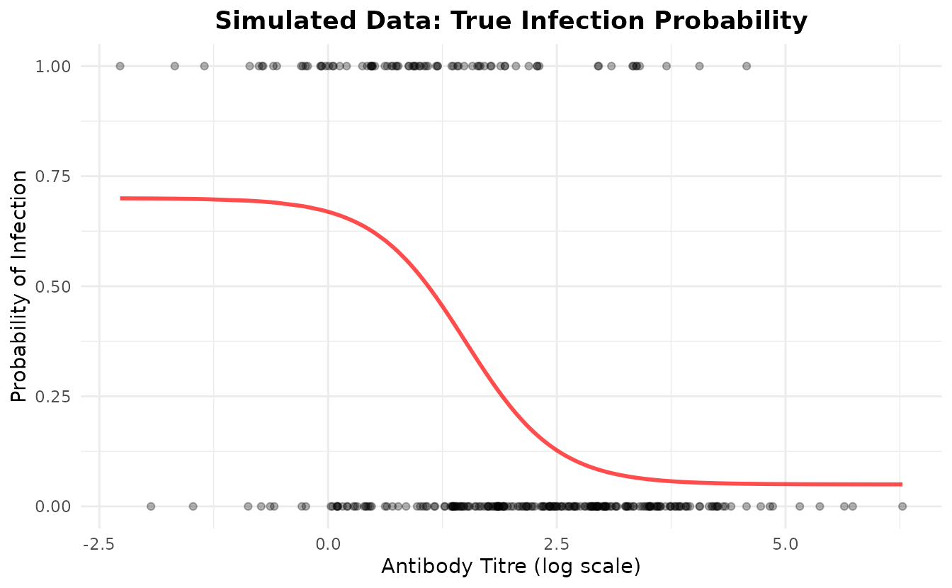
Fit the Model
Now we’ll create a SeroCOP object and fit the Bayesian
model to our simulated data.
Setting Priors
The seroCOP package allows you to customize prior
distributions. By default:
- ec50 is centered at the midpoint of the observed titre range
- ec50_sd is set to titre_range / 4
- floor ~ Beta(1, 9) - weak prior favoring low residual risk at high titres (strong protection)
- ceiling ~ Beta(9, 1) - weak prior favoring high infection risk at low titres
- slope ~ Normal(0, 2) - weakly informative, truncated at 0
# Initialize SeroCOP object
model <- SeroCOP$new(
  titre = sim_data$titre,
  infected = sim_data$infected
)
#> SeroCOP initialized with 300 observations
#>   Infection rate: 27.3%
#>   Titre range: [-2.27, 6.28]

# View default priors (automatically set based on data)
cat("Default priors:\n")
#> Default priors:
print(model$priors)
#> $floor_alpha
#> [1] 1
#>
#> $floor_beta
#> [1] 9
#>
#> $ceiling_alpha
#> [1] 9
#>
#> $ceiling_beta
#> [1] 1
#>
#> $ec50_mean
#> [1] 2.002654
#>
#> $ec50_sd
#> [1] 2.138259
#>
#> $slope_mean
#> [1] 0
#>
#> $slope_sd
#> [1] 2
You can customize priors if you have prior knowledge:
# Example: Set custom priors (not run in this vignette)
model$definePrior(
  floor_alpha = 2, floor_beta = 18,      # Stronger prior: E[floor] ≈ 0.1 (10% residual risk at high titre)
  ceiling_alpha = 18, ceiling_beta = 2,  # Stronger prior: E[ceiling] ≈ 0.9 (90% risk at low titre)
  ec50_mean = 2.0, ec50_sd = 1.0,        # Informative prior on ec50
  slope_mean = 0, slope_sd = 1           # More conservative slope
)
Fitting the Model
# Fit the model (using default data-driven priors)
# Note: Using fewer iterations for vignette speed;
# use more (e.g., iter=2000) for real analysis
model$fit_model(
  chains  = 4,
  iter    = 1000,
  warmup  = 500,
  cores   = 1,    # Adjust based on your system
  refresh = 0
)
#> Warning: Bulk Effective Samples Size (ESS) is too low, indicating posterior means and medians may be unreliable.
#> Running the chains for more iterations may help. See
#> https://mc-stan.org/misc/warnings.html#bulk-ess
Model Diagnostics
Parameter Summary
Let’s examine the posterior distributions of the parameters and compare them to the true values:
# Get parameter summary
param_est <- extract_parameters(model, prob = 0.95)
print(param_est)
#>   parameter      mean     median        lower     upper
#> 1     floor 0.0794394 0.07514709  0.003264366 0.1882319
#> 2   ceiling 0.7976989 0.80514135  0.579668753 0.9923265
#> 3      ec50 0.8457242 0.87565133 -0.068102074 1.6261539
#> 4     slope 1.3594123 1.13635618  0.616379401 3.2693185

# Compare to true values
cat("\nTrue Parameters:\n")
#>
#> True Parameters:
cat(sprintf("  floor:   %.3f\n", true_params$floor))
#>   floor:   0.050
cat(sprintf("  ceiling: %.3f\n", true_params$ceiling))
#>   ceiling: 0.700
cat(sprintf("  ec50:    %.3f\n", true_params$ec50))
#>   ec50:    1.500
cat(sprintf("  slope:   %.3f\n", true_params$slope))
#>   slope:   2.000
Parameter Recovery
Let’s visualize how well we recovered the true parameters:
# Create comparison plot
recovery_df <- data.frame(
  parameter = param_est$parameter,
  estimated = param_est$mean,
  lower = param_est$lower,
  upper = param_est$upper,
  true = c(true_params$floor, true_params$ceiling,
           true_params$ec50, true_params$slope)
)

ggplot(recovery_df, aes(x = parameter)) +
  geom_pointrange(aes(y = estimated, ymin = lower, ymax = upper),
                  color = "steelblue", size = 1) +
  geom_point(aes(y = true), color = "red", size = 3, shape = 4) +
  labs(
    title = "Parameter Recovery",
    subtitle = "Blue: Estimated (95% CI) | Red X: True Value",
    x = "Parameter",
    y = "Value"
  ) +
  theme_minimal() +
  theme(plot.title = element_text(hjust = 0.5, face = "bold"),
        plot.subtitle = element_text(hjust = 0.5))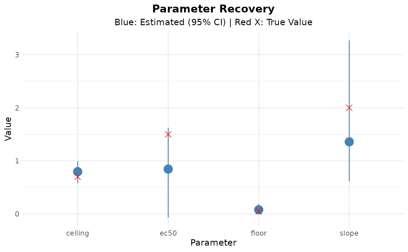
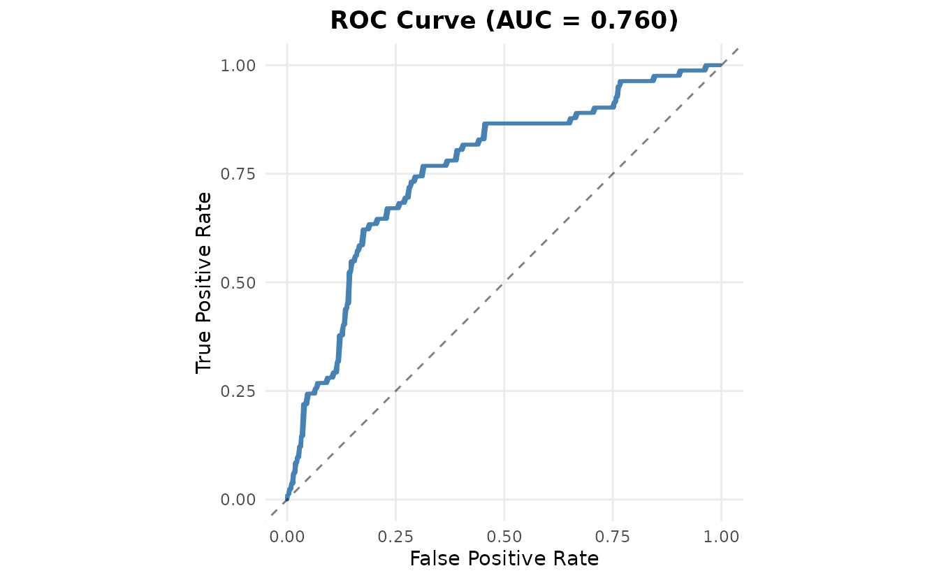
Performance Metrics
Now let’s evaluate the model’s predictive performance:
# Get performance metrics
metrics <- model$get_metrics()
#> Performance Metrics:
#>   ROC AUC (marginalised):        0.760
#>   Brier Score:                   0.164
#>   LOO ELPD:                      -152.67 (SE: 9.16)
The model shows good performance:
- ROC AUC: 0.760 (closer to 1 is better)
- Brier Score: 0.164 (closer to 0 is better)
- LOO ELPD: -152.67 (higher is better)
Visualization
Fitted Curve
model$plot_curve()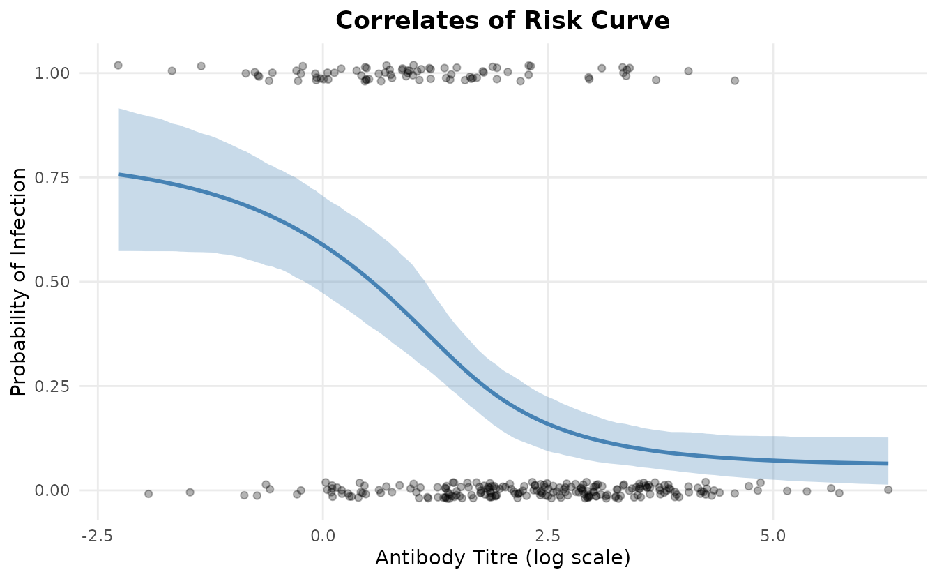
The plot shows:
- Blue line: Posterior mean prediction
- Blue ribbon: 95% credible interval
- Points: Observed infection outcomes (jittered for visibility)
Correlate of Protection
Now let’s extract the correlate of protection directly from the Stan
model. The correlate of protection is calculated within the model as
1 - (prob_infection / ceiling).
# Extract protection probabilities directly from Stan model
protection_samples <- model$predict_protection()
correlate_of_protection <- colMeans(protection_samples)

# Also extract risk for comparison
risk_samples <- model$predict()
correlate_of_risk <- colMeans(risk_samples)

# Display summary
summary_df <- data.frame(
  titre = sim_data$titre,
  correlate_of_risk = correlate_of_risk,
  correlate_of_protection = correlate_of_protection
)

head(summary_df, 10)
#>       titre correlate_of_risk correlate_of_protection
#> 1  2.931135        0.12710867               0.8391943
#> 2  2.053462        0.20936968               0.7334891
#> 3  3.159732        0.11476592               0.8545936
#> 4  3.908734        0.08862574               0.8866631
#> 5  2.556463        0.15413779               0.8049936
#> 6  1.755718        0.25570859               0.6723733
#> 7  2.595668        0.15083593               0.8092037
#> 8  1.880016        0.23501588               0.6997510
#> 9  1.482552        0.30739069               0.6037427
#> 10 3.053227        0.12018647               0.8478490
Correlate of Protection Curve
# Create prediction grid
titre_grid <- seq(min(sim_data$titre), max(sim_data$titre), length.out = 100)

# Extract protection probabilities from Stan model
cop_matrix <- model$predict_protection(newdata = titre_grid)

# Calculate summary statistics
cop_mean <- colMeans(cop_matrix)
cop_lower <- apply(cop_matrix, 2, quantile, probs = 0.025)
cop_upper <- apply(cop_matrix, 2, quantile, probs = 0.975)

# Create plot data
cop_plot_df <- data.frame(
  titre = titre_grid,
  cop = cop_mean,
  lower = cop_lower,
  upper = cop_upper
)

# Plot
ggplot(cop_plot_df, aes(x = titre, y = cop)) +
  geom_ribbon(aes(ymin = lower, ymax = upper), fill = "steelblue", alpha = 0.3) +
  geom_line(color = "steelblue", linewidth = 1) +
  labs(
    title = "Correlate of Protection Curve",
    x = "Antibody Titre (log scale)",
    y = "Correlate of Protection"
  ) +
  theme_minimal() +
  theme(plot.title = element_text(hjust = 0.5, face = "bold"))
The correlate of protection curve shows how protection increases with antibody titre.
Posterior Predictive Checks
Let’s examine the posterior predictive distribution:
# Get predictions
predictions <- model$predict()

# Calculate prediction intervals
pred_mean <- colMeans(predictions)
pred_lower <- apply(predictions, 2, quantile, probs = 0.025)
pred_upper <- apply(predictions, 2, quantile, probs = 0.975)

# Plot calibration
calib_df <- data.frame(
  observed = sim_data$infected,
  predicted = pred_mean,
  titre = sim_data$titre
)

# Binned calibration plot (unique breaks guards against duplicate quantile values)
breaks <- unique(quantile(calib_df$titre, probs = seq(0, 1, 0.1)))
calib_df$bin <- cut(calib_df$titre, breaks = breaks, include.lowest = TRUE)

calib_summary <- aggregate(
  cbind(observed, predicted) ~ bin,
  data = calib_df,
  FUN = mean
)

ggplot(calib_summary, aes(x = predicted, y = observed)) +
  geom_point(size = 3, color = "steelblue") +
  geom_abline(slope = 1, intercept = 0, linetype = "dashed") +
  labs(
    title = "Calibration Plot",
    x = "Predicted Probability",
    y = "Observed Proportion"
  ) +
  theme_minimal() +
  theme(plot.title = element_text(hjust = 0.5, face = "bold")) +
  coord_equal(xlim = c(0, 1), ylim = c(0, 1))
Cross-Validation
The Leave-One-Out Cross-Validation (LOO-CV) provides an estimate of out-of-sample predictive performance:
# Print LOO details
print(model$loo)
#>
#> Computed from 2000 by 300 log-likelihood matrix.
#>
#>          Estimate   SE
#> elpd_loo   -152.7  9.2
#> p_loo         3.3  0.3
#> looic       305.3 18.3
#> ------
#> MCSE of elpd_loo is 0.1.
#> MCSE and ESS estimates assume MCMC draws (r_eff in [0.3, 0.9]).
#>
#> All Pareto k estimates are good (k < 0.7).
#> See help('pareto-k-diagnostic') for details.
Key LOO metrics:
- elpd_loo: Expected log pointwise predictive density
- p_loo: Effective number of parameters
- looic: LOO information criterion (lower is better)
Conclusion
This vignette demonstrated:
- ✅ Simulating data from a four-parameter logistic model
- ✅ Fitting the Bayesian model using the
SeroCOPR6 class - ✅ Recovering true parameter values with credible intervals
- ✅ Calculating performance metrics (ROC AUC, Brier score, LOO-CV)
- ✅ Visualizing results with diagnostic plots
The seroCOP package provides a complete workflow for
correlates of protection analysis with proper uncertainty quantification
through Bayesian inference.
Session Info
sessionInfo()
#> R version 4.5.3 (2026-03-11)
#> Platform: x86_64-pc-linux-gnu
#> Running under: Ubuntu 24.04.3 LTS
#>
#> Matrix products: default
#> BLAS:   /usr/lib/x86_64-linux-gnu/openblas-pthread/libblas.so.3
#> LAPACK: /usr/lib/x86_64-linux-gnu/openblas-pthread/libopenblasp-r0.3.26.so;  LAPACK version 3.12.0
#>
#> locale:
#>  [1] LC_CTYPE=C.UTF-8       LC_NUMERIC=C           LC_TIME=C.UTF-8
#>  [4] LC_COLLATE=C.UTF-8     LC_MONETARY=C.UTF-8    LC_MESSAGES=C.UTF-8
#>  [7] LC_PAPER=C.UTF-8       LC_NAME=C              LC_ADDRESS=C
#> [10] LC_TELEPHONE=C         LC_MEASUREMENT=C.UTF-8 LC_IDENTIFICATION=C
#>
#> time zone: UTC
#> tzcode source: system (glibc)
#>
#> attached base packages:
#> [1] stats     graphics  grDevices utils     datasets  methods   base
#>
#> other attached packages:
#> [1] ggplot2_4.0.2 seroCOP_0.1.0
#>
#> loaded via a namespace (and not attached):
#>  [1] gtable_0.3.6          tensorA_0.36.2.1      xfun_0.57
#>  [4] bslib_0.10.0          QuickJSR_1.9.0        processx_3.8.6
#>  [7] inline_0.3.21         lattice_0.22-9        callr_3.7.6
#> [10] ps_1.9.1              vctrs_0.7.2           tools_4.5.3
#> [13] generics_0.1.4        stats4_4.5.3          parallel_4.5.3
#> [16] tibble_3.3.1          pkgconfig_2.0.3       brms_2.23.0
#> [19] Matrix_1.7-4          checkmate_2.3.4       RColorBrewer_1.1-3
#> [22] S7_0.2.1              desc_1.4.3            distributional_0.7.0
#> [25] RcppParallel_5.1.11-2 lifecycle_1.0.5       compiler_4.5.3
#> [28] farver_2.1.2          stringr_1.6.0         textshaping_1.0.5
#> [31] Brobdingnag_1.2-9     codetools_0.2-20      htmltools_0.5.9
#> [34] sass_0.4.10           bayesplot_1.15.0      yaml_2.3.12
#> [37] pillar_1.11.1         pkgdown_2.2.0         jquerylib_0.1.4
#> [40] cachem_1.1.0          StanHeaders_2.32.10   bridgesampling_1.2-1
#> [43] abind_1.4-8           nlme_3.1-168          posterior_1.6.1
#> [46] rstan_2.32.7          tidyselect_1.2.1      digest_0.6.39
#> [49] mvtnorm_1.3-6         stringi_1.8.7         dplyr_1.2.0
#> [52] labeling_0.4.3        fastmap_1.2.0         grid_4.5.3
#> [55] cli_3.6.5             magrittr_2.0.4        loo_2.9.0
#> [58] pkgbuild_1.4.8        withr_3.0.2           scales_1.4.0
#> [61] backports_1.5.0       rmarkdown_2.30        matrixStats_1.5.0
#> [64] gridExtra_2.3         ragg_1.5.2            coda_0.19-4.1
#> [67] evaluate_1.0.5        knitr_1.51            rstantools_2.6.0
#> [70] rlang_1.1.7           Rcpp_1.1.1            glue_1.8.0
#> [73] pROC_1.19.0.1         jsonlite_2.0.0        R6_2.6.1
#> [76] systemfonts_1.3.2     fs_2.0.0