serosolver guide

Getting started

Overview

serosolver jointly infers antibody kinetics, infection histories and attack rates from cross-sectional or longitudinal serological data, originally described by Kucharski et al. [1] and developed further by Hay et al. [2] . serosolver exploits the predictability of antibody kinetics over time following exposure, using one or more antibody level measurements combined with an antibody kinetics model to back-calculate (i.e., extrapolate backwards) the timing of individual infections.

What distinguishes serosolver from other time-since-infection models is a) jointly inferring an antibody kinetics model and infection histories within the same framework; b) the ability to infer multiple infections per person; and c) supporting multi-antigen systems as well as single-antigen problems.

The core of the package is the serosolver function, which takes all of the data and model assumptions as inputs and saves Markov chain Monte Carlo (MCMC) outputs to disk. serosolver implements a flexible, hierarchical model, meaning that users must be aware of a number of model design decisions. In this vignette, we will show how longitudinal, multi-strain serological data can be cleaned for use in serosolver, and walk through the core functionality of the package and post-processing functions. It is a long vignette, but worth stepping through to make sure you understand how this fairly complex model works!

Contents

This guide provides an overview of the key components for fitting a serosolver model. For more in depth instructions on specific features and detailed methods, see the case study vignettes. We will discuss the following workflow:

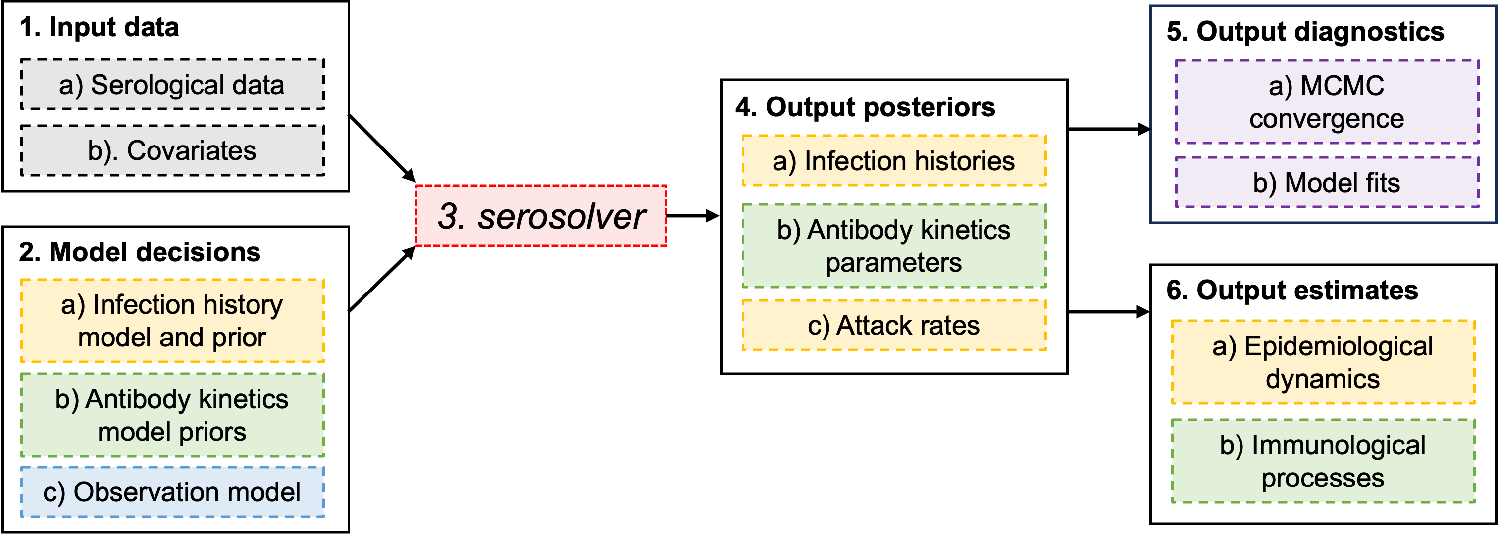
Outline of the serosolver workflow

Entire workflow

The following code runs the entire pipeline for a simulation-recovery experiment with serosolver. We will step through each of these sections in more detail in this guide.

set.seed(123)

library(serosolver)
data(example_par_tab)
data(example_antigenic_map)

## Define a vector of all possible infection times
possible_exposure_times <- seq(2000,2024,by=1)

## Vector of antigens with observations, corresponding to times of circulation
sampled_antigens <- seq(min(possible_exposure_times), max(possible_exposure_times), by=2)

## Times at which serum samples can be taken from individuals
sampling_times <- 2020:2024

## Number of serum samples taken per person
n_samps <- 5

## Simulate some random attack rates
attack_rates <- simulate_attack_rates(possible_exposure_times)

## Use example antigenic map (can also be left as NULL)
antigenic_map <- example_antigenic_map[1:25,]
antigenic_map$inf_times <- possible_exposure_times

## Simulate a full serosurvey with these parameters
all_simulated_data <- simulate_data(par_tab=example_par_tab, group=1, n_indiv=100,
                                    possible_exposure_times=possible_exposure_times,
                                    measured_biomarker_ids = sampled_antigens,
                                    sampling_times=sampling_times, nsamps=n_samps,
                                    antigenic_map=antigenic_map,
                                    age_min=10,age_max=75,
                                    attack_rates=attack_rates, repeats=1,
                                    data_type="continuous")

## Pull out the simulated titre data and infection histories
antibody_data <- all_simulated_data$antibody_data
true_inf_hist <- all_simulated_data$infection_histories
plot_antibody_data(antibody_data,possible_exposure_times,1:4,infection_histories = true_inf_hist)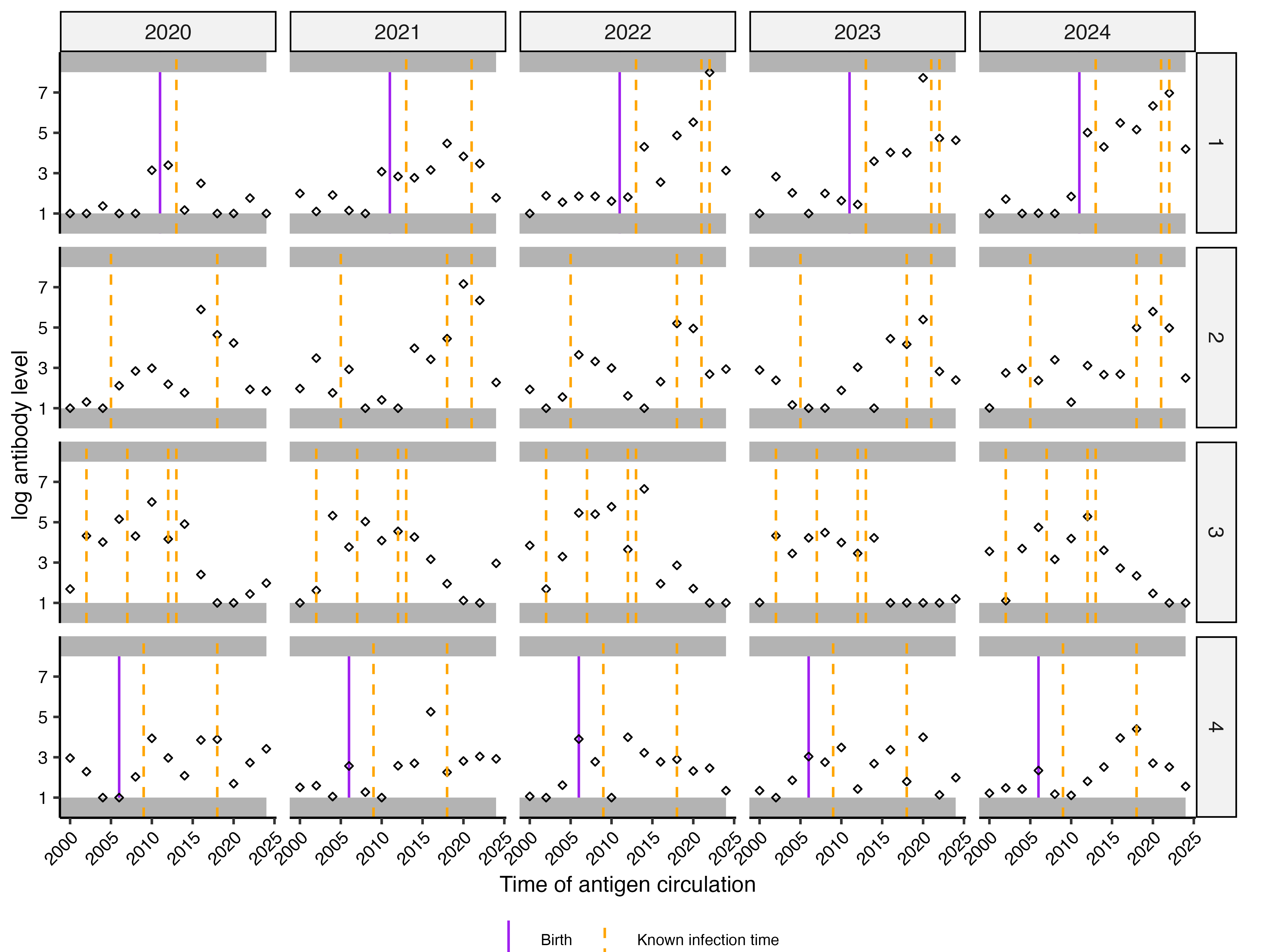

## MCMC settings used by the executable example
mcmc_pars <- c(adaptive_iterations=100000, iterations=200000,
               thin=10, thin_inf_hist=2000, save_block=1000)

res <- serosolver(
  example_par_tab,
  antibody_data,
  antigenic_map = antigenic_map,
  filename = mcmc_file,
  n_chains = 3,
  parallel = TRUE,
  mcmc_pars = mcmc_pars,
  data_type="continuous"
)

Installation and dependencies

Install serosolver using the remotes package:

remotes::install_github("seroanalytics/serosolver")

Note, that serosolver uses Rcpp code, including RcppArmadillo. You will therefore need a working C++ compiler such as clang or gcc. The easiest way to set this up is up for Windows users is the Rtools package. For Mac users, you will need to install a compiler such as Xcode or clang.

The required and additional packages can be installed from CRAN using:

required_packages <- c(
  "data.table", "ggplot2", "dplyr", "tidyr", "Rcpp", "coda",
  "doParallel", "doRNG", "foreach", "Matrix", "MASS", "reshape2",
  "tibble", "RcppArmadillo", "RcppParallel"
)

additional_packages <- c(
  "remotes", "devtools", "plyr", "tidyverse"
)

install.packages(c(required_packages, additional_packages))

Input data

serosolver expects several inputs, including the serological data, a data frame controlling the model parameters (par_tab), an antigenic map or vector of possible exposure times (antigenic_map or possible_exposure_times), and optionally a data frame of demographic data (demographics). This section will walk the users through creating each of these inputs.

Serological data

serosolver expects a data frame of serological data in long format (i.e., there is a row for each observation), referred to as antibody_data in most function arguments, giving the individual ID, sample time, biomarkers or antigens measured, serological measurement, and demographic information:

data(example_antibody_data)
knitr::kable(head(example_antibody_data))

individual	sample_time	birth	repeat_number	biomarker_id	biomarker_group	measurement	population_group
1	2010	1988	1	1968	1	1.69	1
1	2010	1988	2	1968	1	1.00	1
1	2010	1988	1	1972	1	1.00	1
1	2010	1988	2	1972	1	1.00	1
1	2010	1988	1	1976	1	1.00	1
1	2010	1988	2	1976	1	1.39	1

Key point: all variables in serosolver are indexed from 1, matching R coding style rather than C++.

Description of variables:

1. individual: consecutive integer ID of individuals from $1,\dots,N$, where $N$ is the number of individuals in the sample.
2. sample_time: integer value of the time period in which a sample was collected i.e., the observation time.
3. biomarker_id: integer ID of the measured biomarker or antigen, matching entries in antigenic_map.
4. biomarker_group: optional, integer ID of the measurement type. Set this to 1 when all measurements are the same kind. Use different numbers when each sample contains different kinds of measurements, such as an antibody titre and an avidity measurement.
5. measurement: the measurement for this individual against biomarker_id at sample_time i.e., the observation.
6. repeat_number: integer value starting from 1 where repeat measurements are available per sample and biomarker_id combination.
7. population_group: integer ID separating individuals within a sample into different groups (explained below).
8. birth: integer value giving the time period (matching the supported range of sample_time) in which an individual was born i.e., the date of birth.

Data can be cross-sectional samples with multiple biomarkers measured per sample (e.g., multiple influenza strains), such that different biomarker_ids correspond to different time periods, or longitudinal samples with one or more biomarkers measured per sample (e.g., measuring measles IgG titers over time).

Use check_data() to check that the required columns and values are present before fitting a model. The examples in this guide use the supplied example_antibody_data dataset.

Serological data should be inspected before fitting with:

plot_antibody_data(example_antibody_data,example_antigenic_map$inf_times,n_indivs=1:3,study_design = "cross-sectional")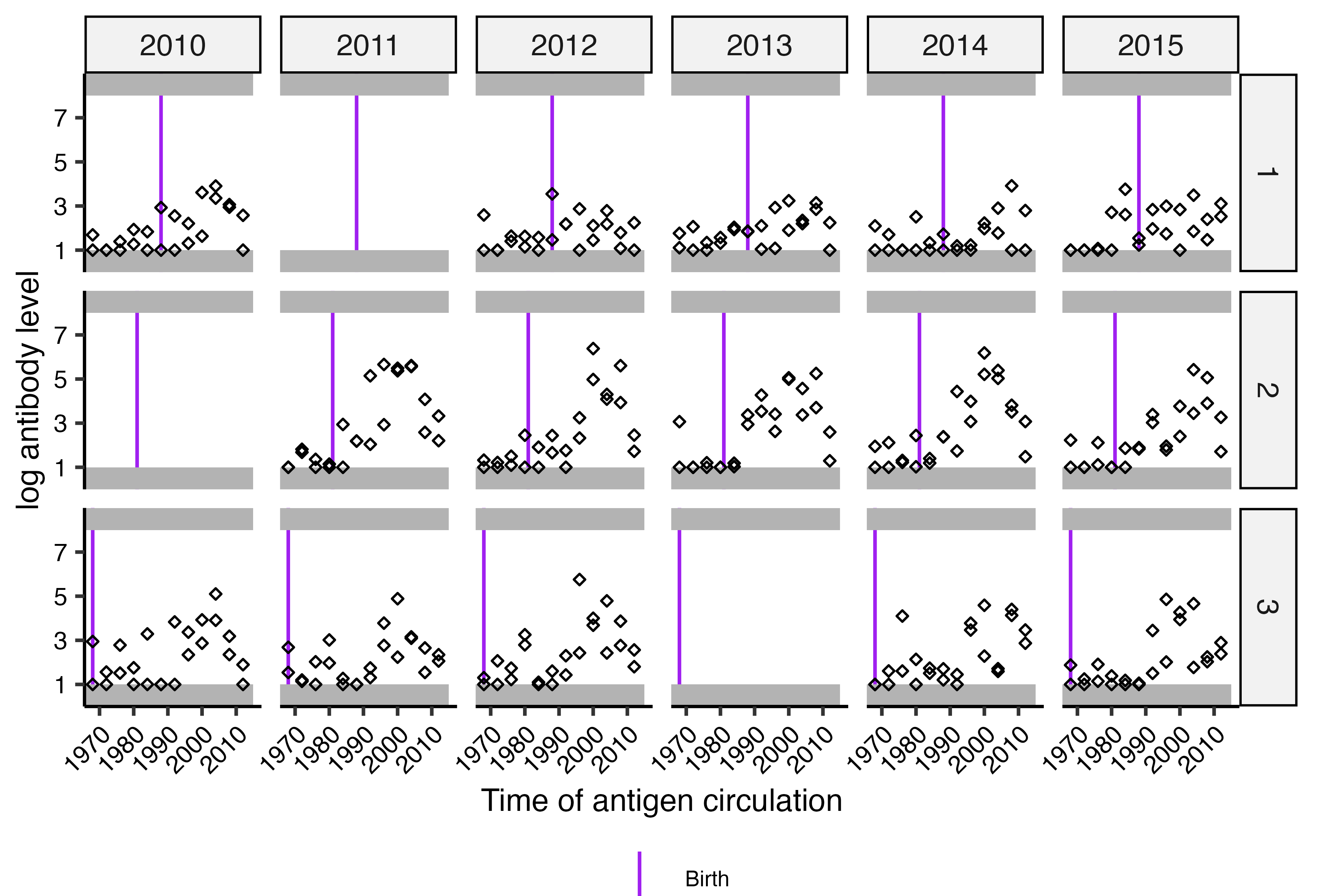

Cross-sectional serology against multiple antigens from multiple serum samples. Plot columns give time periods of sample times, rows give individuals. X-axis gives the time each biomarker ID was assumed to be circulating.

plot_antibody_data(dplyr::filter(example_antibody_data, biomarker_id %in% c(1968,2004,2012)),2010:2015,n_indivs=1:3,study_design = "longitudinal")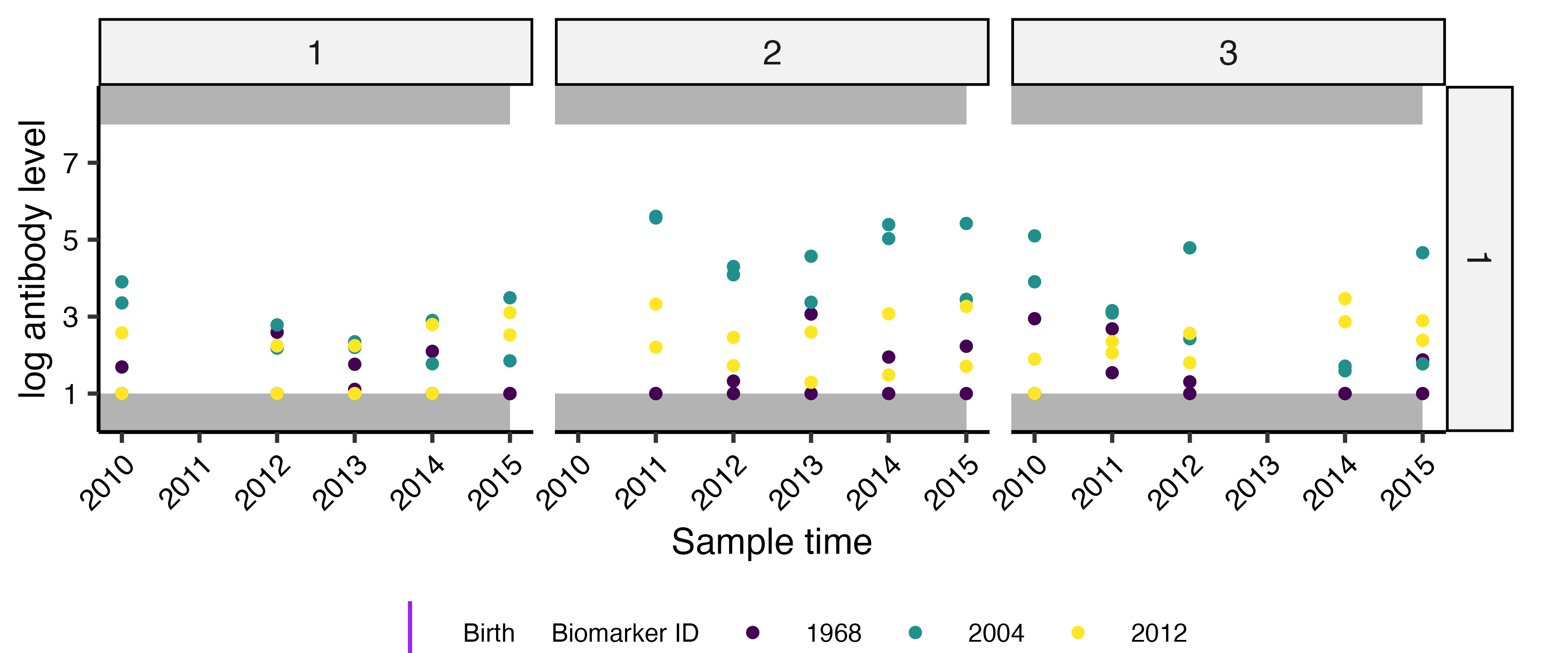

Longitudinal serology against multiple antigens from multiple serum samples. Plot columns give individuals, rows give biomarker groups (not biomarker IDs!). Points are coloured by biomarker ID. X-axis gives time of sample collection.

Antigenic map

serosolver was designed to treat biomarker_id as interchangeable with the time variables, such that one antigen ID is assumed to circulate in one time period. For example, biomarker_id=1968 refers to the antigen assumed to be circulating in 1968. Note that at present, serosolver supports only one antigen/biomarker per time period. However, a single biomarker_id can be assumed to circulate and dominate for multiple time periods, which can be specified by modifying the antigenic_map object.

The antigenic_map object tells serosolver how different biomarker_ids are antigenically related to each other (using coordinates on an antigenic map), as well as the time periods during which the biomarker_id is assumed to be circulating. Antigenic maps are commonly used to quantitatively represent antigenic relationships between antigenically variable pathogens [3]. Setting all antigenic coordinates to the same values tells serosolver that there are no antigenic differences between biomarker_ids (i.e., no antigenic variation). The same thing can be achieved by setting antigenic_map=NULL and instead specifying the possible_exposure_times vector.

## Example antigenic map
data(example_antigenic_map)
knitr::kable(head(example_antigenic_map))

inf_times	x_coord	y_coord
1968	334	255
1969	335	254
1970	335	253
1971	336	252
1972	337	252
1973	338	251

## Antigenic map with no antigenic variation
data.frame(x_coord=1,y_coord=1,inf_times=1:10)

## Antigenic map with clusters, each one circulated for 3 time units
data.frame(x_coord = rep(seq(1,3,by=1),each=3), y_coord=rep(seq(1,3,by=1),each=3),inf_times=1:9)

## Antigenic map with two biomarker groups
data.frame(x_coord=1,y_coord=1,inf_times=rep(1:10,2),biomarker_group=rep(c(1,2),each=10))

Covariate data

Individuals can’t be infected before they’re born, and we can’t infer infections which occurred after the final sample from each individual. serosolver uses the birth and sample_time variables to constrain when and which biomarker_ids an individual can have been infected by.

The population_group variable is used to split individuals into groups under different infection rates. These might represent different geographic groups or demographic groups. For example, we might be interested in comparing attack rates and infection histories between two locations with very different epidemiological dynamics. In this case, we shouldn’t assume that all individuals are under the same force of infection, and thus we need to tell serosolver to account for this difference in two places:

## Set individual 1:25 to population_group 1, and individual IDs >25 to population_group 2
antibody_data <- antibody_data %>% mutate(population_group=if_else(individual <= 25, 1, 2))

par_tab[par_tab$names %in% c("infection_model_prior_shape1","infection_model_prior_shape2"),"stratification"] <- "population_group"

For most simple models, this variable can be ignored or set to 1 for all individuals and par_tab$stratification can be left as NA.

Similar logic can be applied to stratify the antibody kinetics by one or more covariates. For example, we might want to test if antibody titres wane quicker in certain age groups. The general approach is similar to population_group:

## Split into two age groups based on whether the individual was born on or before 1990 or after
antibody_data <- antibody_data %>% mutate(age_group=if_else(birth <= 1990, 1, 2))

## Tell serosolver to stratify the wane_short parameter by age_group
par_tab[par_tab$names == "wane_short","stratification"] <- "age_group"

There are a few ways the user can implement this depending on their desired model (e.g., should covariates be static over the study period or change with e.g., age?). Demographic information can be supplied in a separate dataset. Covariates can be static, such as sex or location, or can change over time, such as age group or vaccination status. Multiple covariates can also be combined when defining groups, allowing the model to compare infection rates or antibody kinetics across more detailed demographic categories. These features are explained in the demographic variables and covariates vignette.

serosolver can also estimate different antibody kinetics for different variants or strains that circulated at different times. This follows a slightly different workflow, because the grouping is linked to the infection or exposure variant rather than directly to the individual, and is also explained in the demographic variables and covariates vignette.

The parameter table (par_tab)

par_tab is the model control object. It contains one row for each model parameter and tells serosolver which values to use, which values to estimate, and the allowed ranges.

The main columns are:

1. names: the parameter names used by the model.
2. values: the parameter value supplied to the model. This is used as the starting value when random_start_parameters = FALSE in the serosolver function call; otherwise, estimated parameters start with values generated using lower_start and upper_start.
3. fixed: set to 1 to keep a parameter fixed, or 0 to estimate it during the MCMC run.
4. lower_bound and upper_bound: the lowest and highest values allowed during model fitting.
5. lower_start and upper_start: the range used when generating random starting values for estimated parameters. You can tighten these bounds to ensure serosolver starts with plausible parameter values.
6. stratification: the name of a column used when a parameter should vary between groups. Leave this as NA when no groups are needed.
7. biomarker_group: identifies which type of measurement the parameter belongs to. This should match the values in antibody_data.

The optional steps column controls the initial proposal step size for an estimated parameter. The infection-history prior also requires parameters named infection_model_prior_shape1 and infection_model_prior_shape2. There is also the par_type, variable, which is an internal label used to organise model parameters, such as antibody parameters, infection-history parameters, and measurement offsets. This can be ignored by the user.

The supplied example shows the expected structure:

data(example_par_tab)
knitr::kable(example_par_tab)

## Check the table before fitting
checked_par_tab <- check_par_tab(example_par_tab)

Parameters can be changed by selecting their names. For example, this fixes the short-term waning parameter at 0.25:

par_tab[par_tab$names == "wane_short", "values"] <- 0.25
par_tab[par_tab$names == "wane_short", "fixed"] <- 1

Model decisions

Before fitting a model, think about the timescale and range of infection times that you would like to estimate and the features of the antibody kinetics model you’d like to fit. These choices determine how serosolver interprets the dataset and the resulting estimates. In particular, make sure that all time variables use the same reference and resolution, and that assay limits and measurement types are correctly represented in par_tab.

Infection history model and priors

One of the most confusing model design decision in serosolver is setting the infection history model. First, we need to understand the epidemiological question we seek to address. If our main objective is to estimate attack rates, we need to think about the power/information we have to estimate attack rates and infection histories at a chosen time resolution (e.g., annual attack rates or per month). If instead our main objective is to understand antibody kinetics, we might wish to simplify the infection history model to allow a more complex antibody kinetics model. The rationale is the same as any other statistical model: practical parameter identifiability is limited by the data, and thus we should choose as simple a model structure as possible to answer our question.

Model time resolution

It is possible to estimate infection states just for the duration of the serostudy, or to estimate infection histories for an arbitrary number of time periods prior to the study. For example, we might use serosolver to estimate infections that occurred between two serum sample collection times in the same way we would measure seroconversion rates. Alternatively, we might only have serum samples for recent time periods, but aim to estimate infection histories all the way back to the time of birth.

All time variables in a serosolver model must be at the same time resolution, including sample_time, biomarker_id, birth, and possible_exposure_times. This can cause confusion, as these variables must be integers, and thus we have to do some transformation before running serosolver:

• For annual samples, the sample time is simply the year each sample was collected in. For example, data collected between 2009 and 2011 would simply have values of 2009, 2010, or 2011.

• For semi-annual samples, the sample time is the year the sample was collected multiplied by 2 (since there are two time periods in each year). For example, data collected between 2009 and 2011 would have values of $(2009 \times 2) + 1 = 4019$, $(2009.5 \times 2) + 1 = 4020$, $(2010 \times 2) + 1 = 4021$, $(2010.5 \times 2) + 1 = 4022$, $(2011 \times 2) + 1 = 4023$, $(2011.5 \times 2) + 1 = 4024$.

• Similarly, for quarterly or monthly samples, the sample time follows the same pattern. For example for a sample collected in July of 2009, the quarterly sample time would be $(2009 + \frac{3}{4})\times 4 + 1 = 8040$ (because July is in the third quarter of the year) and the monthly sample time would be $(2009 + \frac{7}{12})\times12 + 1 = 24116$ (because July is the seventh month).

serosolver estimates an infection state for each element of the vector possible_exposure_times, which is either passed directly or extracted automatically from antigenic_map$inf_times. The range and entries of these vectors therefore determines the model time period and resolution of the infection history model. If antigenic_map is specified, then you can typically leave possible_exposure_times as NULL. If you aren’t using an antigenic map, then you must specify possible_exposure_times.

## possible_exposure_times is used in multiple places to tell serosolver the vector of times at which individuals might be infected
possible_exposure_times <- seq(2000,2025,by=1) ## Annual infection states
possible_exposure_times <- seq(2000*4, 2025*4,by=1) ## Quarterly infection states

## antigenic_map contains the same information as possible_exposure_times in its inf_times variable
possible_exposure_times <- antigenic_map$inf_times

A useful feature of serosolver is to use mixed time resolutions. For example, we might estimate infection histories at an annual resolution up to 2009, and then at a per-quarter resolution thereafter. Another example might be to estimate per-cluster infections for historic periods of time to establish long-term infection histories, and then per-quarter or per-year infection histories during the study period to model shorter-term dynamics. This can be useful for reducing parameter space when we have limited information to draw inferences about particular time periods, but rich information for others:

## Infection states every 4 years up to 2020, then yearly
possible_exposure_times <- c(seq(1990, 2019,by=4), seq(2020,2025,by=1))

Infection history priors

A very important consideration, but one which is highly technical and unimportant for most users, is the structure of the prior to place on the individual infection histories. Most of the supplementary material of the main publication is about this decision.

For most users, the only thing you need to consider is the prior you wish to place on the per-time probability of infection. As individual infection states are modeled as Bernoulli variables (i.e., they can be 0 or 1), an appropriate prior for the per-time probability of infection is a Beta distribution. Thus, by changing the shape parameters of this Beta distribution, we can change the prior on the infection states. For example, we might want to use uninformative priors by setting both shape parameters to 1. Alternatively, we might have some prior understanding of the probability of infection in each time period — if we think the annual attack rate is around 5%, we might set the Beta distribution shape parameters to 0.5 and 10 (which would give a mean prior attack rate of 5%); try hist(rbeta(1000, 0.5, 10)).

Note that serosolver assumes the same Beta prior applies to all individuals and all time periods by default, so choose your Beta parameters carefully. However, it is possible to use a separate Beta prior for different population groups, for example, if you want to model the fact that individuals in different locations are under independent forces of infection. This is referenced in 1.3 Covariate data and illustrated in the case study guides.

It is possible to assume different priors for the infection history model, but this is complex and not necessary for most use cases. You can read more about the different priors in the main publication, and if you really know what you’re doing you can change the prior model with the prior_version argument of the main serosolver function.

Antibody kinetics model and priors

serosolver models antibody measurements as arising from antibody responses following one or more infections. Users can specify the size and timing of short- and long-term boosts, antibody waning, antigenic seniority, and cross-reactivity between biomarkers using an antigenic map. The model is described fully in the main publication. In the parameter file, the column fixed indicates if each parameter value is fixed (fixed=1) or should be estimated (fixed=0). A brief summary of each model level is described here.

You can inspect the assumed antibody kinetics model using the plot_antibody_model function along with par_tab, the antigenic map, and a chosen infection history. For example, the current assumed antibody kinetics model using the example antigenic map and assuming a single infection in 1975 produces longitudinal antibody kinetics and antibody landscapes which look like this:

#> [[1]]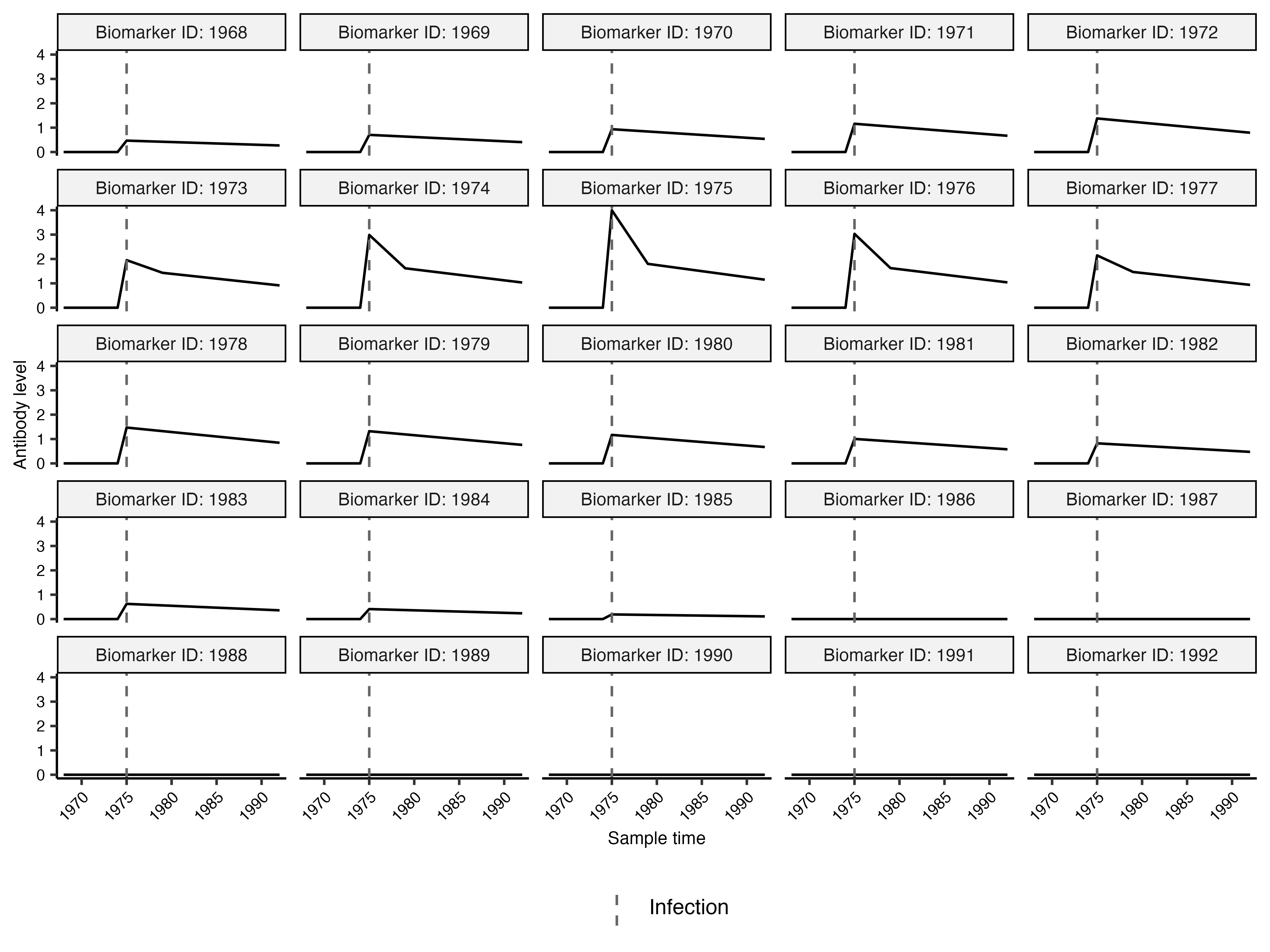

#> 
#> [[2]]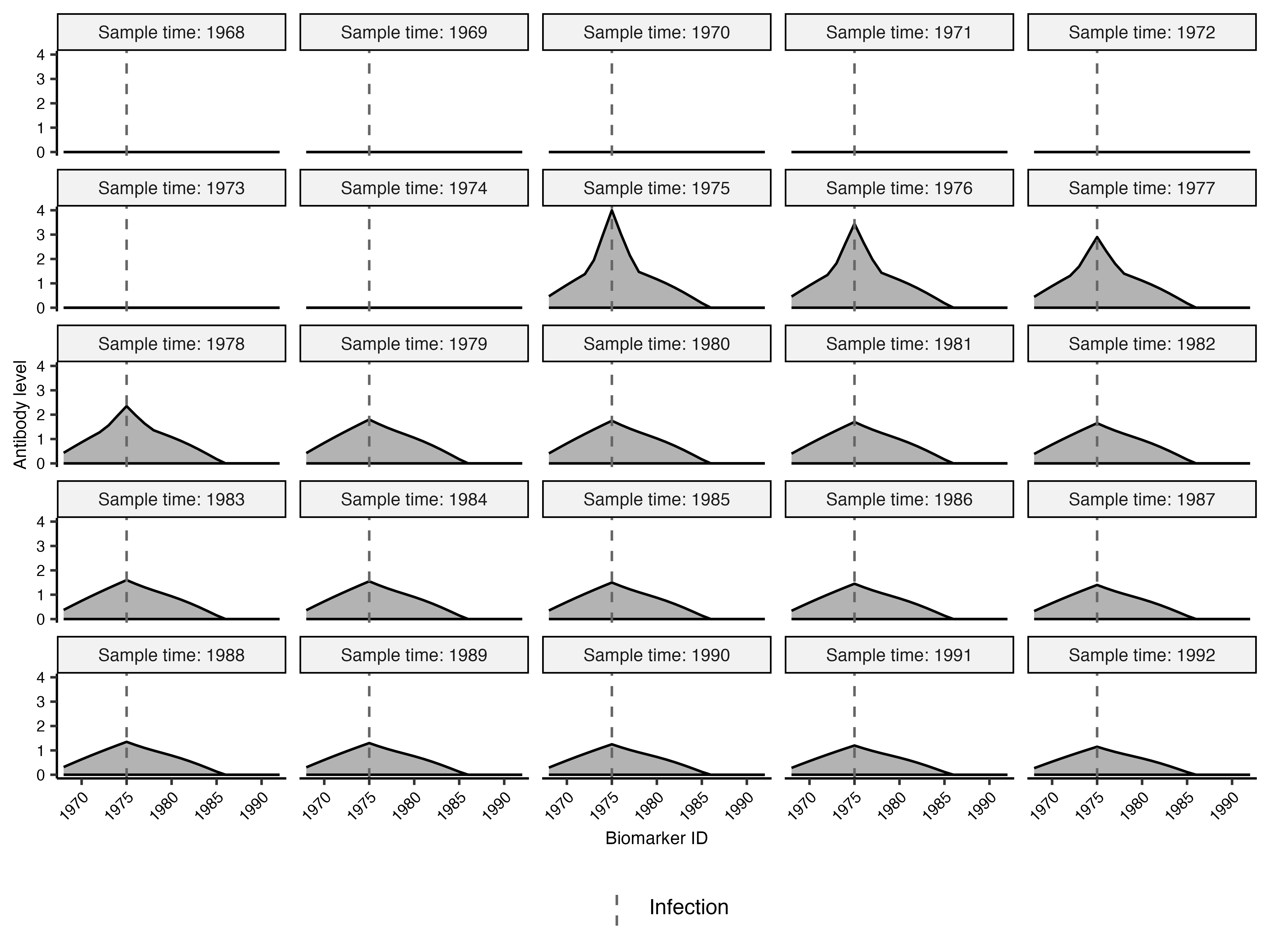

The first plot shows the modelled antibody level over time (on the x-axis) stratified by each biomarker ID in the antigenic map. The second plot shows the antibody landscape at each sample time (as facets) with biomarker ID on the x-axis.

Boosting

Following infection, serosolver assumes that an individual’s antibody level against the infecting strain/variant increases by $\mu_{long} + \mu_{short}$, coded as boost_short + boost_long units over boost_delay time units. Note that boost_delay should be in integer units matching the timescale of the model. Estimating boost_short and boost_long jointly may be challenging without sufficient data, particularly longitudinal data to distinguish a short-term, transient response from the long-term, persistent response. Users may therefore wish to fix one of these parameters either at a known value or at 0.

Waning

Both the short- and long-term boosts can be set to wane over time. These rates are set by $\omega_{short}$ and $\omega_{long}$, coded as wane_short and wane_long respectively. In practice, we have found it difficult to identify both waning rates, and usually fix wane_long at 0. Note that this parameter is not an exponential (on the natural scale) waning rate parameter by default: it describes the proportion of the boost lost per time unit since infection, $t$:

$$W(t)=\max\{0,1-\omega t\}$$

Alternatively, users can model waning as exponential decay on the log scale (so exponential-on-exponential on the natural scale). Add a fixed model-option row named exponential_waning to par_tab, with values = 1 and par_type = 0:

$$W(t) = e^{-\omega t}$$

Note that this setting also changes the cross-reactivity model below. The rationale behind these waning models is described in this publication.

exponential_par_tab <- example_par_tab
exponential_par_tab$values[exponential_par_tab$names == "exponential_waning"] <- 1

plot_antibody_model(
  pars = exponential_par_tab,
  infection_history = 1975,
  antigenic_map = example_antigenic_map,
  times = example_antigenic_map$inf_times[1:25]
)[[1]]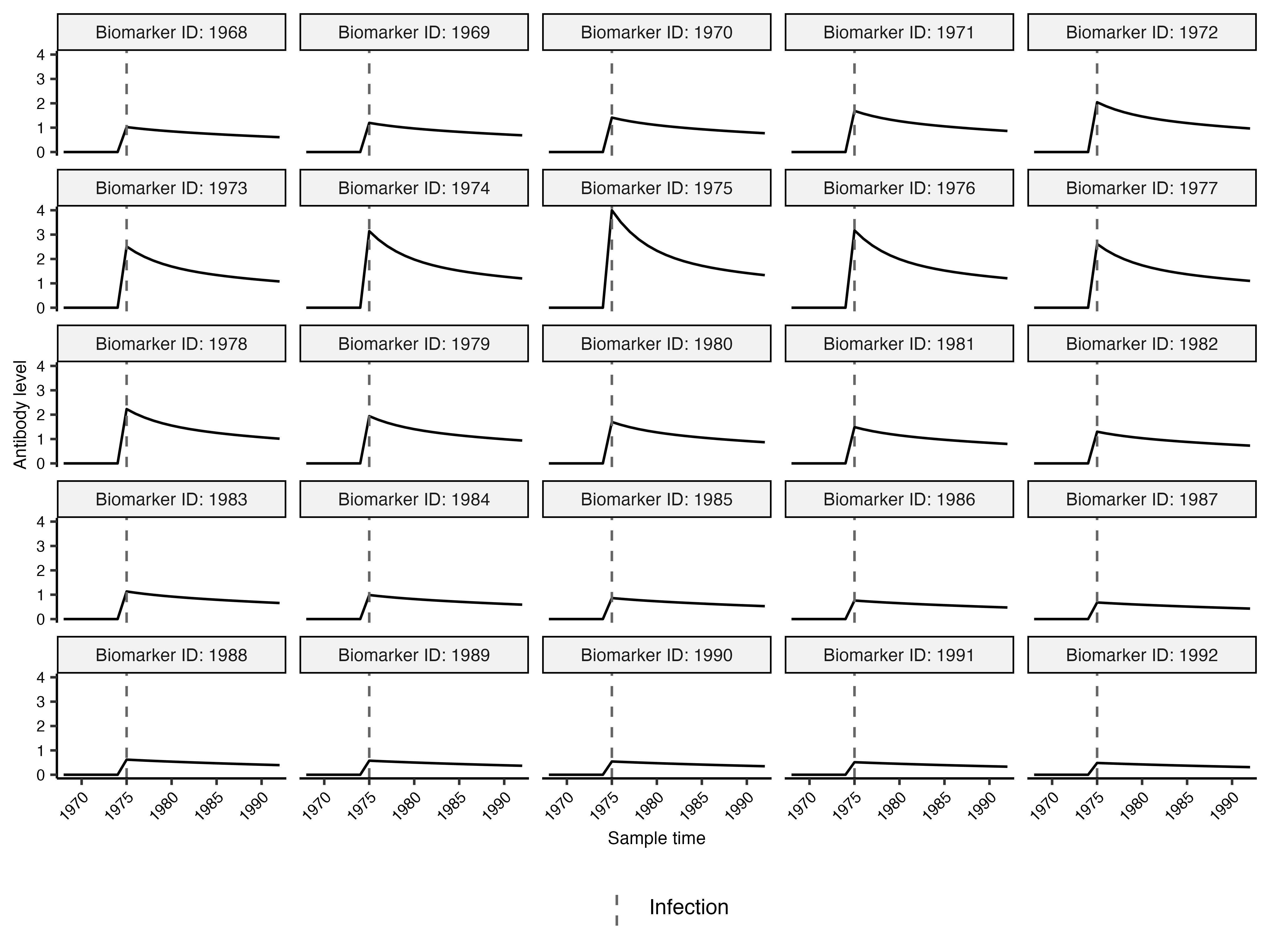

If the exponential_waning row is absent, or its values entry is 0, the model uses linear waning and the waning parameters should be bounded between 0 and 1. With values = 1, the waning parameters should be positively bounded. The old exponential_waning argument remains available for compatibility but is deprecated; the par_tab row takes precedence when both are supplied.

Cross-reactivity

Cross-reactivity between biomarker IDs is modelled using the antigenic map input. Separate cross-reactivity parameters are used for the short- and long-term boosts, usually because short-term boosting is antigenically broader than the long-term boost. Cross-reactivity is modelled as a declining boost with increasing antigenic distance from the infecting strain: the degree of boosting to the infecting strain, $x$, is just boost_long+boost_short, but for heterologous strains, $y$, this declines as a linear function of antigenic distance such that the degree of boosting of antibody levels to strain $y$ given infection with strain $x$ is:

$$B_{x,y}=\mu_{long} \text{max}\{0,1-\sigma_{long} \delta_{x,y}\} + \mu_{short} \text{max}\{0,1-\sigma_{short}\delta_{x,y}\}$$ where $\sigma_{long}$ and $\sigma_{short}$ correspond to cr_long and cr_short in par_tab respectively, and $\delta_{x,y}$ is the Euclidean distance between strain $x$ and strain $y$ calculated from the antigenic map directly.

As with the waning model, cross-reactivity can instead be assumed to decline exponentially rather than linearly with antigenic distance as:

$$B_{x,y}=\mu_{long}e^{-\sigma_{long} \delta_{x,y}} + \mu_{short}e^{-\sigma_{short} \delta_{x,y}}$$

If the linear form is used, the cross-reactivity parameters should be bounded between 0 and 1. With the exponential form selected in par_tab, the cross-reactivity parameters should be positively bounded.

If fixing either the long-term or short-term boosting arms to 0, then it is recommended to also fix the corresponding cross-reactivity parameters at 0.

Antigenic seniority

serosolver can model the overall level of antibody boosting to decline with each successive infection using the antigenic seniority parameter, $\tau$, or antigenic_seniority. Antigenic seniority is modelled here as a simple phenomenological effect and thus we caution against overinterpretation. It simply suppresses each successive boost as a function of the number of prior infections as:

$$S(k) = \text{max}\{0, 1-\tau(k-1)\}$$

where $k-1$ gives the number of infections prior to the current one. Thus, the first infection has $S_{1}=1$, the second has $S(2)=\text{max}\{0, 1-\tau\}$, and the third has $S(3)=\text{max}\{0, 1-2\tau\}$, etc. Setting $\tau=0$ means that there is no reduction. This model stems from the paper by Kucharski et al and should not be over-interpreted as mechanistically representing antigenic seniority, back-boosting, or antibody ceiling effects.

Observation model

Most applications of serosolver involve fitting to antibody titre or concentration data. The model asumes that observations are distributed around some true value predicted by the model i.e., it accounts for observation noise.

serosolver accommodates both continuous and discrete data, and accounts for the upper and lower limits of detection of the assay. Continuous data can take values across a range, whereas discrete data take separate values such as integer titre categories. These limits and the measurement type will need to be specified in the model using the par_tab object. serosolver also supports multiple measurement types per sample, for example, measuring both antibody titre and avidity (see the advanced features vignette). These observation types are distinguished by the biomarker_group variable – all observations within a biomarker_group are underpinned by their own antibody kinetics model parameters, but arising from the same individual-level infection histories.

The following inputs should be updated depending on the limits of detection of the assay used and whether the data are continuous or discrete:

## Example of two biomarker_groups, one has discrete data one has continuous data
## Set bounds of the assay
par_tab[par_tab$names=="min_measurement" & par_tab$biomarker_group == 1,"values"] <- 0
par_tab[par_tab$names=="max_measurement" & par_tab$biomarker_group == 1,"values"] <- 10

par_tab[par_tab$names=="min_measurement" & par_tab$biomarker_group == 2,"values"] <- 1
par_tab[par_tab$names=="max_measurement" & par_tab$biomarker_group == 2,"values"] <- 8

## Set observation type: discrete, continuous, or continuous with false positives
data_type <- c("discrete", "continuous", "false_positive") ## used in `serosolver::serosolver`, `serosolver::simulate_data` etc

Priors

The prior distributions should be checked before fitting the model. This is useful for checking that the model gives reasonable weight to the infection histories, attack rates, and antibody kinetics that you consider plausible.

Fixed and estimated parameters

The fixed column in par_tab controls whether a value is kept fixed or estimated by MCMC. Set fixed = 1 when a value is known or is being held at a chosen value, and set fixed = 0 when the value should be estimated. Fixed values do not have posterior uncertainty. For an estimated parameter, values is the starting value when random_start_parameters = FALSE; when random starting values are used, lower_start and upper_start are used to generate the starting value.

For example, this fixes the short-term waning parameter at 0.25:

par_tab[par_tab$names == "wane_short", "values"] <- 0.25
par_tab[par_tab$names == "wane_short", "fixed"] <- 1

Bounds in par_tab

lower_bound and upper_bound are hard limits for an estimated parameter. MCMC proposals outside these limits are not accepted. They therefore restrict the range over which a prior can put weight, but they are not prior means or standard deviations. The lower_start and upper_start columns only control random starting values and do not define the prior.

The bounds should match the parameter scale. For example, a probability is usually bounded between 0 and 1, while a positive antibody boost can have a lower bound of 0 and a larger upper bound. The bounds also determine the transformation used internally for many parameters, so they should be set before fitting and checked with check_par_tab().

Antibody-kinetics parameter priors

The prior_func argument can be used to specify prior distributions for the antibody-kinetics parameters. It is an outer function that receives par_tab once and returns a function that receives the current parameter values during the MCMC run. The returned function should return one log-prior value, usually by adding the log densities for the parameters to which priors have been assigned.

For example, the following uses log-normal priors for positive parameters and a Beta prior for a parameter bounded between 0 and 1:

prior_func <- function(par_tab) {
  par_names <- as.character(par_tab$names)
  boost_long <- which(par_names == "boost_long")
  boost_short <- which(par_names == "boost_short")
  wane_short <- which(par_names == "wane_short")
  obs_sd <- which(par_names == "obs_sd")

  function(pars) {
    names(pars) <- par_names
    sum(
      dlnorm(pars[boost_long], log(2), 0.5, log = TRUE),
      dlnorm(pars[boost_short], log(2), 0.5, log = TRUE),
      dbeta(pars[wane_short], 4, 8, log = TRUE),
      dlnorm(pars[obs_sd], log(1), 0.5, log = TRUE)
    )
  }
}

The function is passed to serosolver(prior_func = prior_func). If a parameter is stratified, include every generated coefficient row in the prior function; this is illustrated in the demographic variables and covariates vignette.

Infection-history shape priors

For most users, the prior on the per-time probability of infection is defined by the two rows named infection_model_prior_shape1 and infection_model_prior_shape2. If these values are $\alpha$ and $\beta$, the per-time infection probability has a Beta distribution:

$$p_t \sim \operatorname{Beta}(\alpha, \beta), \qquad E[p_t] = \frac{\alpha}{\alpha + \beta}.$$

The sum $\alpha + \beta$ controls how concentrated the prior is around its mean. For example, alpha = 0.5 and beta = 10 gives a prior with mean about 5% and places substantial weight near low probabilities. The same Beta prior is applied across people and exposure times unless it is stratified by population_group or another demographic variable.

The corresponding prior can be inspected with rbeta():

prior_attack_rate <- rbeta(10000, 0.5, 10)
hist(prior_attack_rate, breaks = 50,
     main = "Prior attack rate", xlab = "Per-time probability of infection")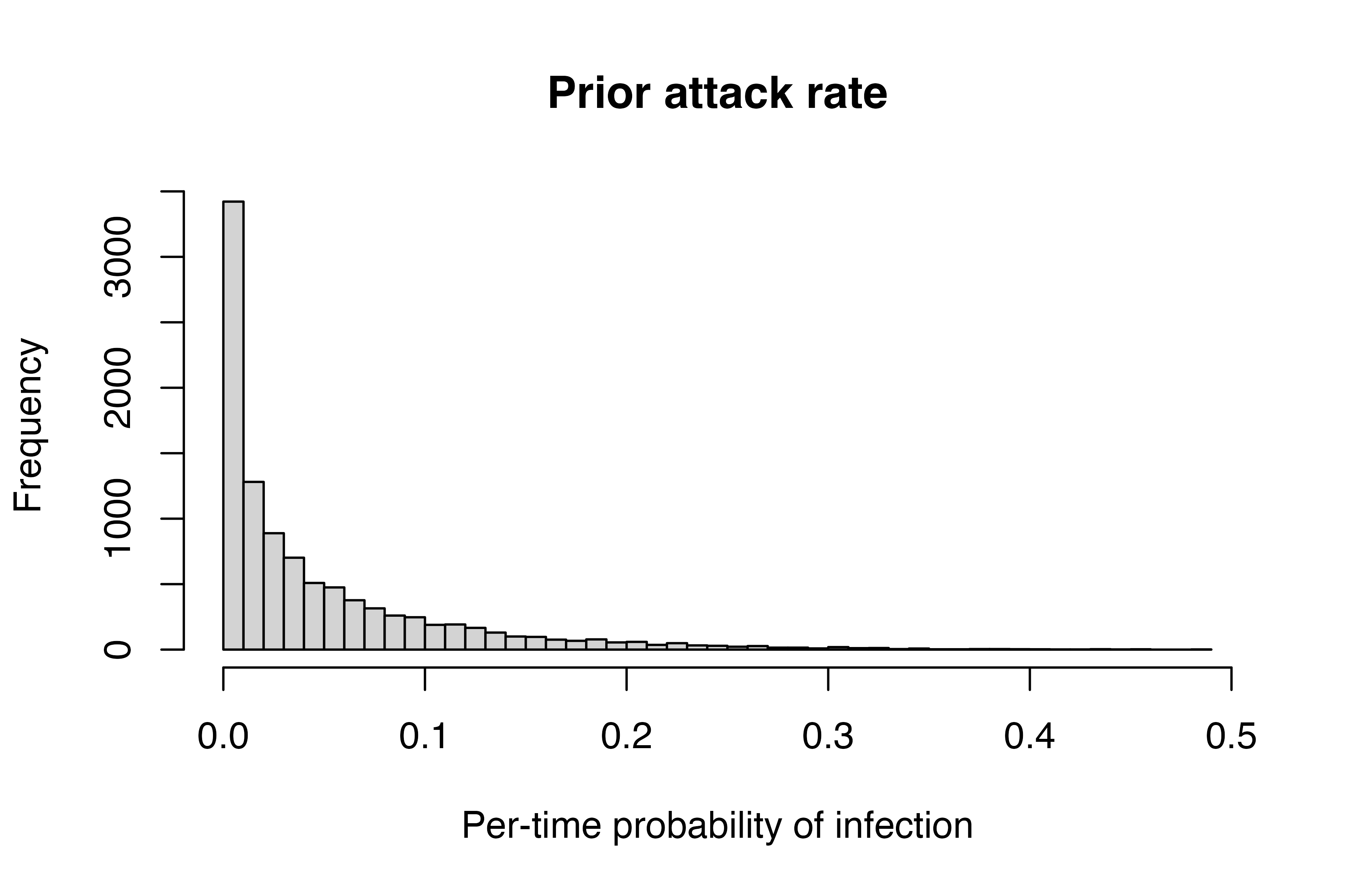

Under the default prior version 2, the attack rates shown after fitting are calculated from the inferred infection histories. They are therefore realised sample proportions implied by those histories, rather than direct draws of the Beta parameters. Prior version 1 instead estimates a separate phi for each exposure time; this distinction is demonstrated in the advanced features vignette.

Sampling from the priors

Set solve_likelihood = FALSE to run the MCMC without using the antibody observations in the likelihood. This samples from the specified parameter and infection-history priors, allowing prior predictive checks before fitting the data. The resulting chains can be inspected with the usual plotting and summary functions, for example:

prior_fit <- serosolver(
  par_tab = par_tab, antibody_data = antibody_data,
  antigenic_map = example_antigenic_map,
  possible_exposure_times = possible_exposure_times,
  prior_func = prior_func, solve_likelihood = FALSE,
  filename = "prior_predictive", n_chains = 3,
  parallel = TRUE, mcmc_pars = mcmc_pars
)

plot_attack_rates(
  prior_fit$mcmc_chains$inf_chain,
  settings = prior_fit$settings
)

This separates the assumptions made before seeing the data from the posterior results obtained after the likelihood is included.

Advanced features

serosolver has a number of advanced features for greater control over the model assumptions and inputs. Users can fix selected infection states, provide starting antibody levels, include measurement offsets (for systematic measurement biases), use exponential rather than linear antibody waning, and fit multiple biomarker groups such as antibody titre and avidity together.

These features require additional data preparation and model decisions. They are explained in detail in the advanced features vignette and the relevant case-study material.

Running serosolver

After much data cleaning and model decision making, you are ready to pass your data and model inputs into serosolver. The main serosolver() function runs a custom, adaptive Metropolis-Within-Gibbs algorithm to sample from the posterior distribution for the model parameters given the input data. In other words, it estimates the antibody kinetics model parameters and infection histories in a Bayesian framework. Attack rates are calculated from these infection-history draws. The function saves the draws to files and returns a list containing the saved-file locations, model settings, diagnostics, and plots when these are requested.

Using the default options, the serosolver can be run using:

res <- serosolver(par_tab = par_tab, antibody_data = antibody_data, antigenic_map = antigenic_map)

Users should modify the mcmc_pars argument to make adjustments for run time, convergence, and MCMC chain storage. This will mainly come down to increasing or decreasing the number of iterations and the adaptive period, though there are a number of fine-tuning inputs described in the details of ?serosolver.

mcmc_pars <- c("iterations"=50000,"target_acceptance_rate_theta"=0.44,"target_acceptance_rate_inf_hist"=0.44,
              "adaptive_frequency"=1000,"thin"=1,
              "adaptive_iterations"=10000, "save_block"=1000,
              "thin_inf_hist"=100, "proposal_inf_hist_indiv_prop"=0.5,
              "proposal_ratio"=2, "proposal_inf_hist_time_prop"=0.5,
              "proposal_inf_hist_distance"=5, "proposal_inf_hist_adaptive"=0,
              "proposal_inf_hist_indiv_swap_ratio"=0.5,"proposal_inf_hist_group_swap_ratio"=0.5,
              "proposal_inf_hist_group_swap_prop"=0.5)
res <- serosolver(par_tab = start_tab, titre_dat = titre_dat, antigenic_map = antigenic_map,
              mcmc_pars = mcmc_pars,data_type="continuous")

MCMC output is written to files automatically. The filename argument provides the prefix of the file names; _chain.csv and _infection_histories.csv are appended for the parameter and infection-history chain files. When multiple chains are run in parallel, progress messages are written to a matching _log.txt file in the same directory. A settings file is also saved alongside the chains to easily read back in all of the model inputs and settings.

The vignette uses saved chain output when it is available, so normal builds do not rerun the MCMC. If the saved output is absent, knitting the complete guide runs the model and may take several minutes.

To read the saved chains and serosolver_settings back into R, point load_mcmc_chains() to the directory containing the files:

chains <- load_mcmc_chains(
  location = mcmc_dir,
  par_tab = example_par_tab,
  burnin = 500,
  thin = 1,
  convert_mcmc = TRUE
)
## Load the input settings
load(paste0(mcmc_file, "_serosolver_settings.RData"))

Output posteriors

serosolver generates numerous plots to visualise results and evaluate model performance. The vast majority of these are generated automatically by the serosolver() function as part of the return object. A few examples are shown below, but take a look at all of the objects in the list returned by serosolver():

print(res$plot_fits_cross_sectional[[1]])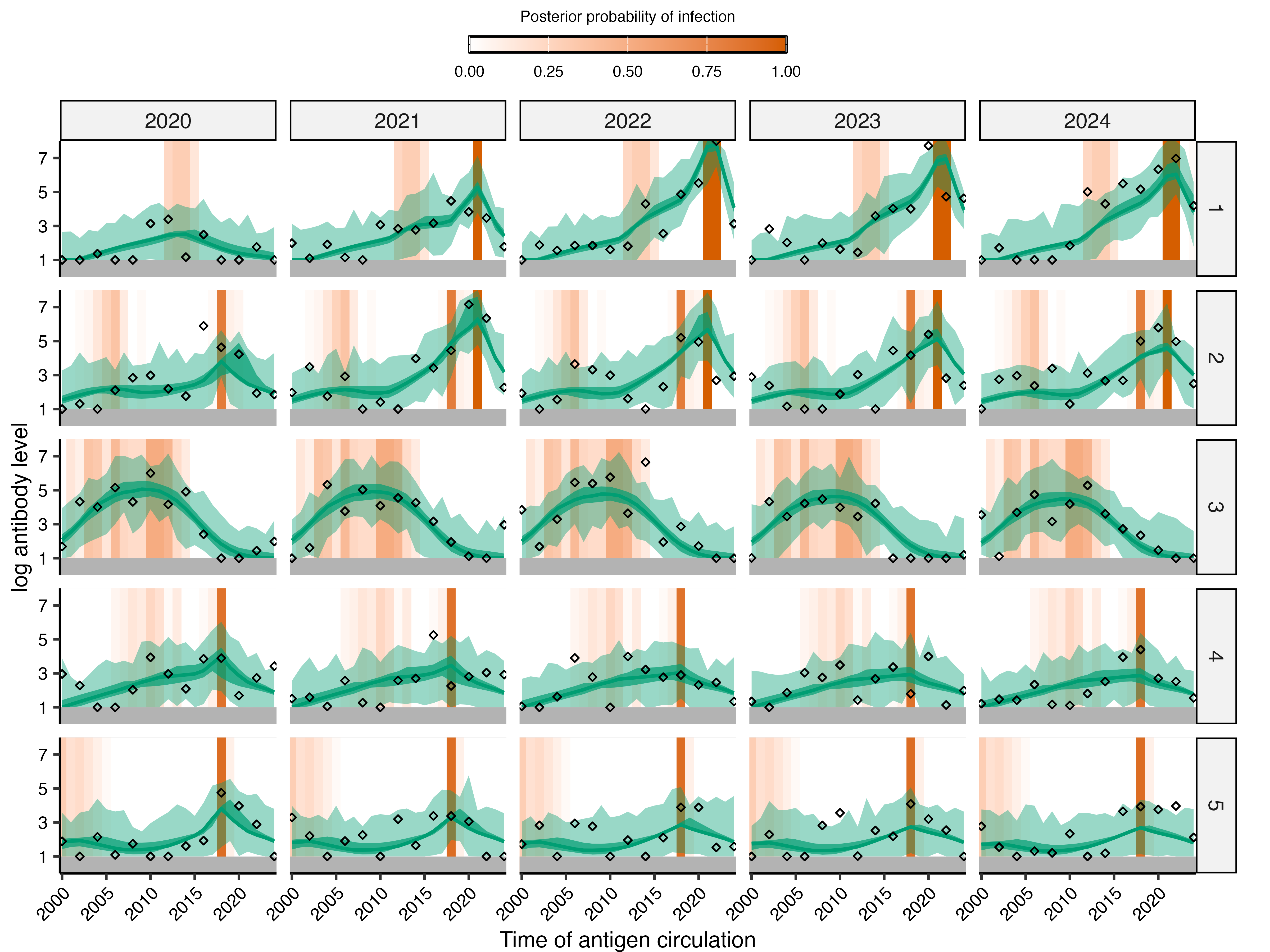

Model fits to the first 5 individuals, plotted as cross-sectional data. Each column depicts a sample time, each row depicts an individual. The x-axis shows the biomarker_id corresponding to the antigenic map. Black diamonds show observations, green lines/shaded regions show posterior median/95% credible intervals/95% prediction intervals. Orange bars show the inferred infection times – darker orange denotes greater posterior probability.

print(res$plot_attack_rates)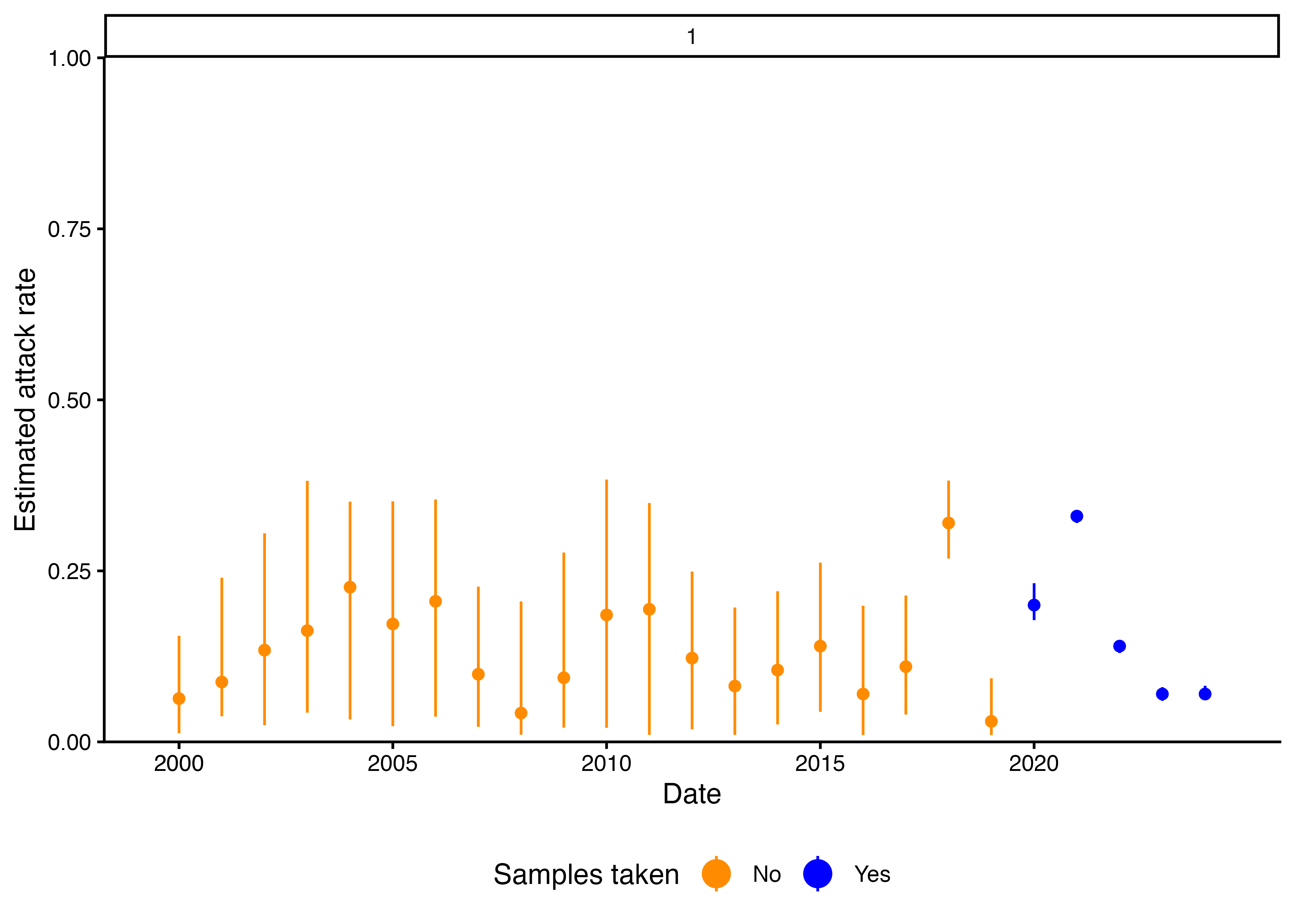

Estimated population attack rates over time. The facet shows population_group. X-axis shows time, and the y-axis shows the per-capita attack rate per time unit. Pointrange plots show posterior medians and 95% CrI. Note that the time periods are coloured by whether or not observations were made in that time period (i.e., older time periods are informed by back-calculating historic infections).

print(res$plot_antibody_model)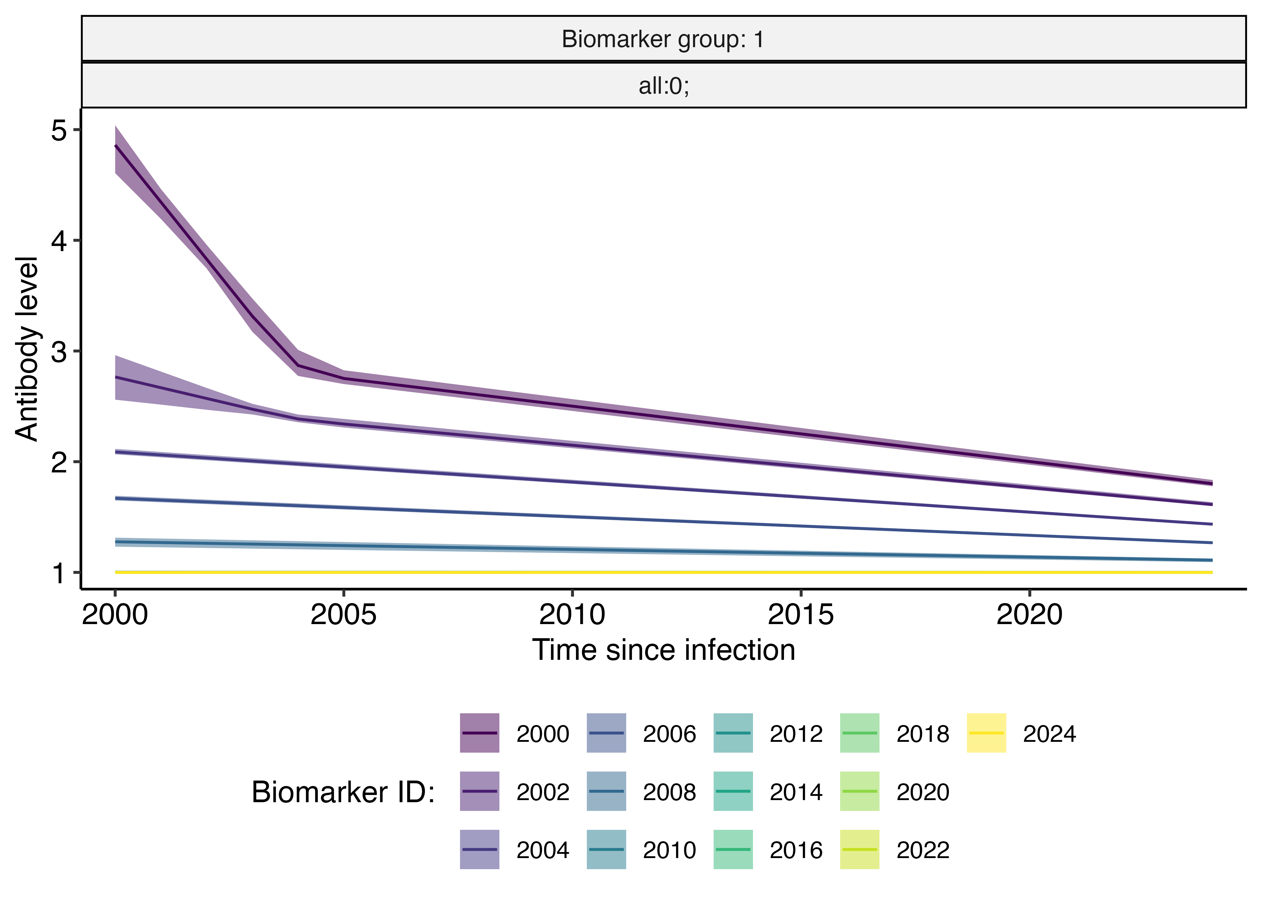

Estimated antibody kinetics model over time-since-infection. The lines/shaded regions show posterior median/95% CrI estimates. The facets are used to group estimates by biomarker_group and covariate group (universal groups in this example). In this example, each colour represents a different biomarker ID, and the example assumes a single infection at t=2000 (i.e., the plot shows cross-reactive boosting and waning).

These plots are generated automatically by serosolver(), but they can also be reproduced manually from the saved chains. This is useful when you want to change the number of plotted individuals, samples, burn-in, or other plotting options without rerunning the model. The chains and settings loaded in Section 3 are used in the following examples:

Further details about MCMC settings, including save_block and thin_inf_hist, are available in the serosolver help file. The load_mcmc_chains() help file describes the returned chain objects.

The same plotting functions used internally by serosolver() can be called directly:

plot_model_fits(
  chains$theta_chain, chains$inf_chain,
  settings = serosolver_settings,
  individuals = 1:5,
  orientation = "cross-sectional"
)

plot_attack_rates(chains$inf_chain, settings = serosolver_settings)

plot_estimated_antibody_model(
  chains$theta_chain,
  settings = serosolver_settings,
  solve_times = serosolver_settings$possible_exposure_times
)

To compare the observed measurements with predictions from individual posterior draws, use plot_antibody_predictions(). The p_hist_draws plot shows the observations alongside a random selection of posterior draws, with a separate facet for each draw. This gives a visual check of the variation represented by the fitted observation model, rather than only showing the posterior median.

prediction_plots <- plot_antibody_predictions(
  chain = chains$theta_chain,
  infection_histories = chains$inf_chain,
  settings = serosolver_settings,
  nsamp = 100
)
print(prediction_plots$p_hist_draws)
#> `stat_bin()` using `bins = 30`. Pick better value `binwidth`.
#> `stat_bin()` using `bins = 30`. Pick better value `binwidth`.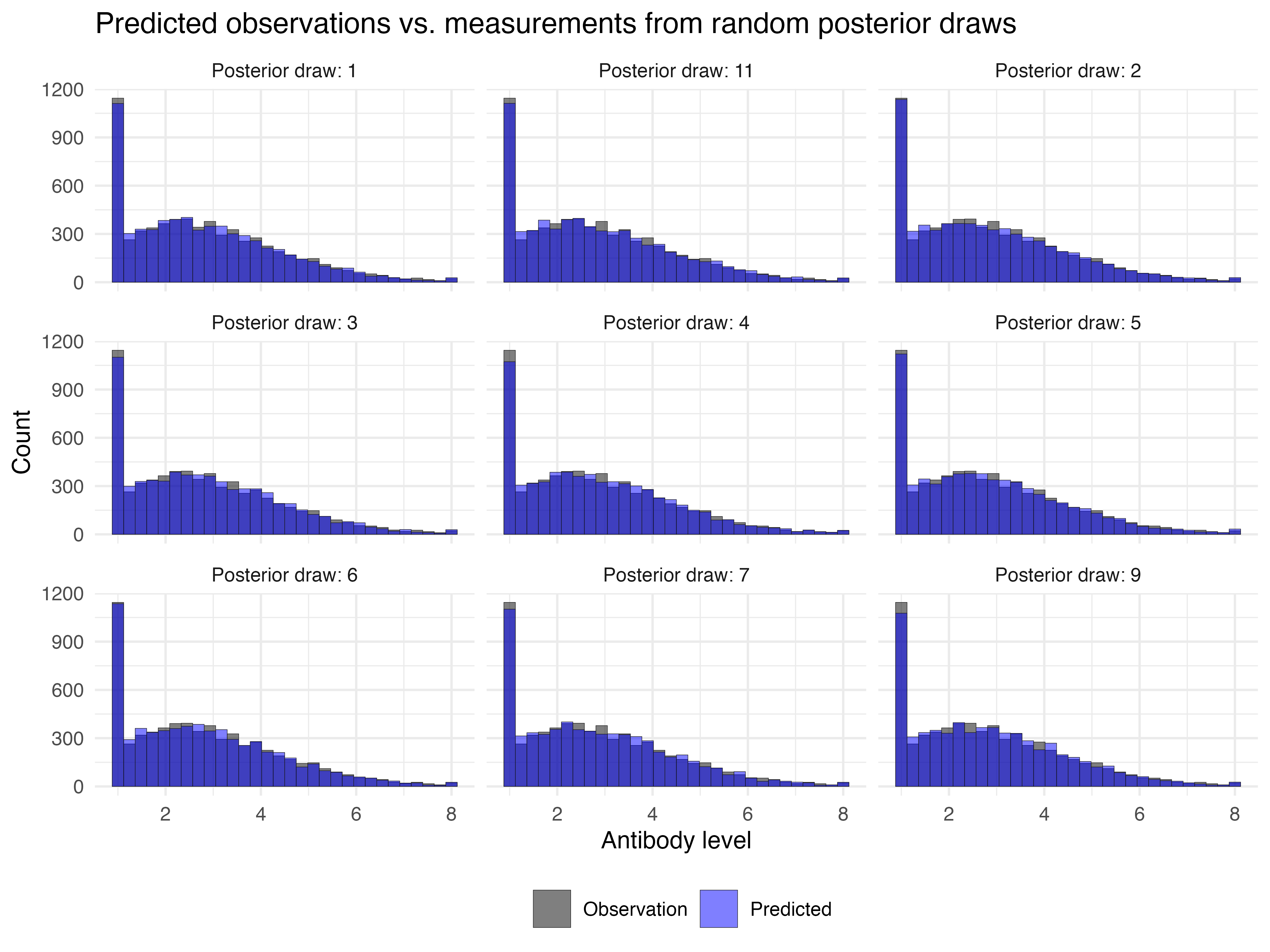

Observed antibody measurements compared with predictions from randomly selected posterior draws.

Both approaches are shown because the returned plots are the quickest way to inspect a fit, whereas reading the chains and calling the plotting functions directly gives more control over post-processing and plotting.

Output diagnostics

To evaluate model performance, trace and density plots should be produced by plotting the MCMC chains. In the below example the adaptive period and burn-in from the MCMC are excluded in the diagnostic plots.

These checks follow typical Bayesian modelling best practice: burn-in is discarded, posterior and prior predictive checks are recommended, chains are compared using R-hat, and effective sample size (ESS) is considered when judging whether estimates are reliable. Because serosolver uses a less efficient MCMC sampler than methods such as Stan, we generally use somewhat more relaxed criteria for R-hat and ESS (roughly R-hat < 1.1 and ESS > 200). The Stan reference manual provides a useful general explanation of these diagnostics. In general, if the model has failed to pass these convergence thresholds, the chains must be re-run with more iterations. Often you will need to increase the number of iterations run by an order of magnitude to go from non-converging chains to converging chains.

print(res$all_diagnostics$p_thetas[[1]] +
        ggplot2::theme(axis.text.x = ggplot2::element_text(angle = 45, hjust = 1)))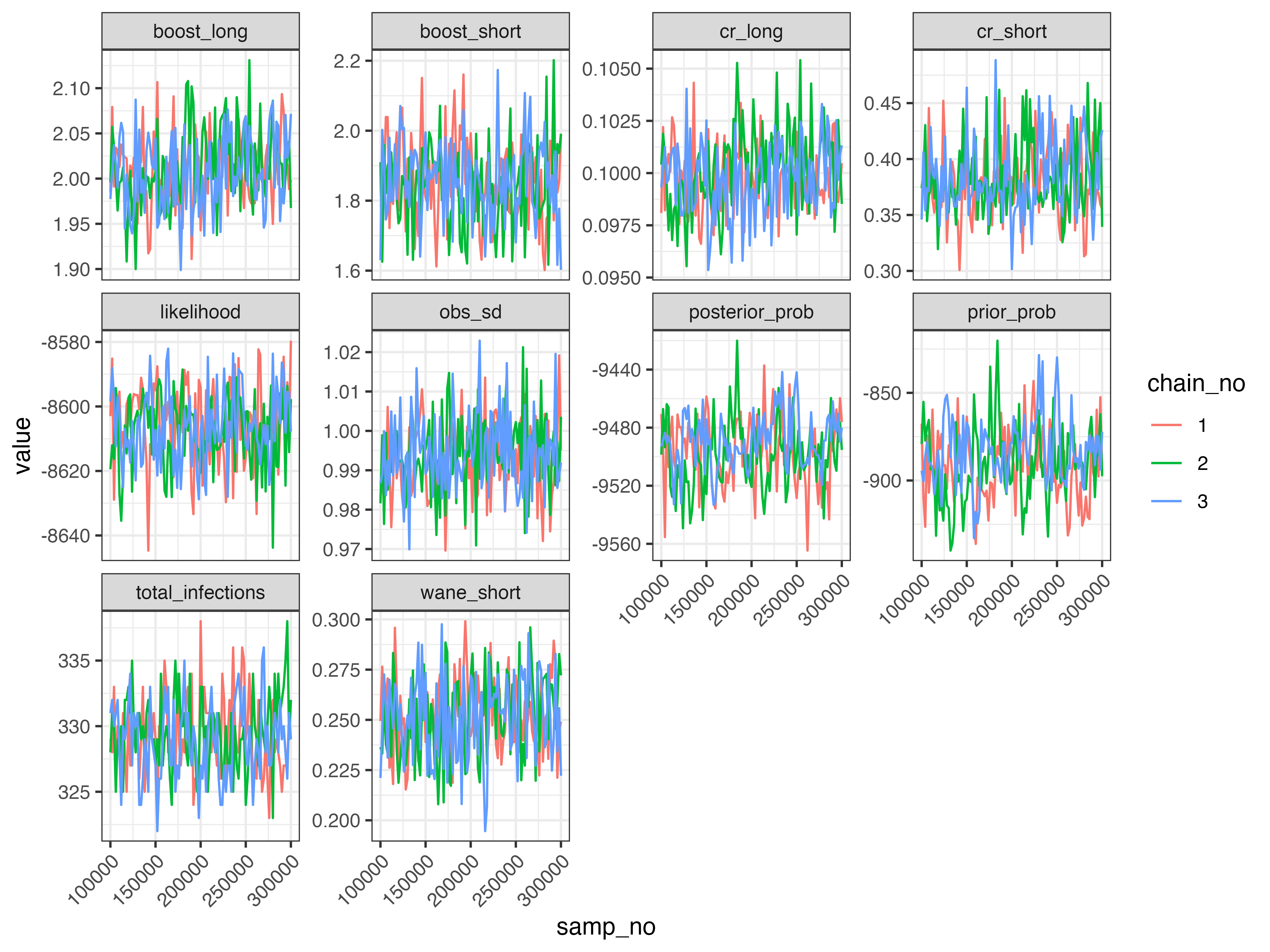

print(res$all_diagnostics$p_inf_hists$by_time_trace +
        ggplot2::theme(axis.text.x = ggplot2::element_text(angle = 45, hjust = 1)))
#> NULL

The diagnostics can also be regenerated from the saved files:

diagnostics <- plot_mcmc_diagnostics(
  location = mcmc_dir, par_tab = example_par_tab, burnin = 500
)
print(diagnostics$p_thetas[[1]] +
        ggplot2::theme(axis.text.x = ggplot2::element_text(angle = 45, hjust = 1)))

Output estimates

The fitted parameter estimates are available directly from the returned res object. The antibody kinetics model parameters are returned as:

res$all_diagnostics$theta_estimates
#>               names  median     mean lower95_CrI upper95_CrI   ess
#>              <char>   <num>    <num>       <num>       <num> <num>
#> 1:       boost_long   2.010   2.0100      1.9372       2.089   229
#> 2:      boost_short   1.850   1.8523      1.6285       2.083   303
#> 3:       wane_short   0.252   0.2514      0.2184       0.289   303
#> 4:          cr_long   0.100   0.0999      0.0965       0.103   109
#> 5:         cr_short   0.377   0.3818      0.3256       0.456   244
#> 6:           obs_sd   0.994   0.9940      0.9749       1.015   421
#> 7: total_infections 329.000 329.2112    324.0000     335.000   198
#>    Rhat point estimate Rhat upper CI
#>                  <num>         <num>
#> 1:               1.011          1.05
#> 2:               1.001          1.01
#> 3:               1.014          1.06
#> 4:               1.061          1.19
#> 5:               0.995          1.00
#> 6:               1.000          1.02
#> 7:               0.999          1.02

The same parameter estimates can be obtained from the saved chains. The chains object was created in Section 4:

theta_summary <- summary(coda::as.mcmc.list(chains$theta_list_chains))
theta_summary$statistics

Summaries of the estimated infection histories and attack rates are also returned by serosolver(), where $j$ denotes the time index (with indices matching antigenic_map or possible_exposure_times) and $i$ denotes the individual ID:

## Per-unit-time total number of infections estimated
head(res$all_diagnostics$inf_hist_estimates$by_year)
#> Key: <j, population_group>
#>        j population_group  mean median lower_quantile upper_quantile
#>    <int>            <num> <num>  <num>          <num>          <num>
#> 1:     1                1  5.77      5              0           14.0
#> 2:     2                1  8.93      8              0           26.4
#> 3:     3                1 11.31     11              0           26.0
#> 4:     4                1 15.27     15              0           34.0
#> 5:     5                1 17.46     18              2           33.4
#> 6:     6                1 13.66     13              1           30.0
#>    effective_size gelman_point gelman_upper
#>             <num>        <num>        <num>
#> 1:          192.9        0.992        0.996
#> 2:           71.5        1.018        1.059
#> 3:          102.2        1.033        1.131
#> 4:          130.0        1.082        1.278
#> 5:          101.0        1.041        1.158
#> 6:          146.8        1.008        1.030

## Per-individual total number of infections estimated
head(res$all_diagnostics$inf_hist_estimates$by_indiv)
#> Key: <i>
#>        i  mean median lower_quantile upper_quantile effective_size
#>    <int> <num>  <int>          <num>          <num>          <num>
#> 1:     1  3.01      3              3              3            303
#> 2:     2  3.03      3              3              4            303
#> 3:     3  4.00      4              4              4            303
#> 4:     4  2.00      2              2              2              0
#> 5:     5  1.95      2              1              2            115
#> 6:     6  4.00      4              4              4            303

These can also be calculated directly from the saved infection-history chain. This can be useful for generating more visually informative output plots, for example:

possible_exposure_times <- serosolver_settings$possible_exposure_times

n_alive <- data.frame(
  j = possible_exposure_times,
  population_group = 1,
  n_alive = get_n_alive(
    serosolver_settings$antibody_data,
    possible_exposure_times
  )
)

p_cumu_infs <- plot_cumulative_infection_histories(
  chains$inf_chain,
  indivs=1:3,
  possible_exposure_times=possible_exposure_times,
  nsamp = 100,
  pad_chain = TRUE
)

print(p_cumu_infs[[1]])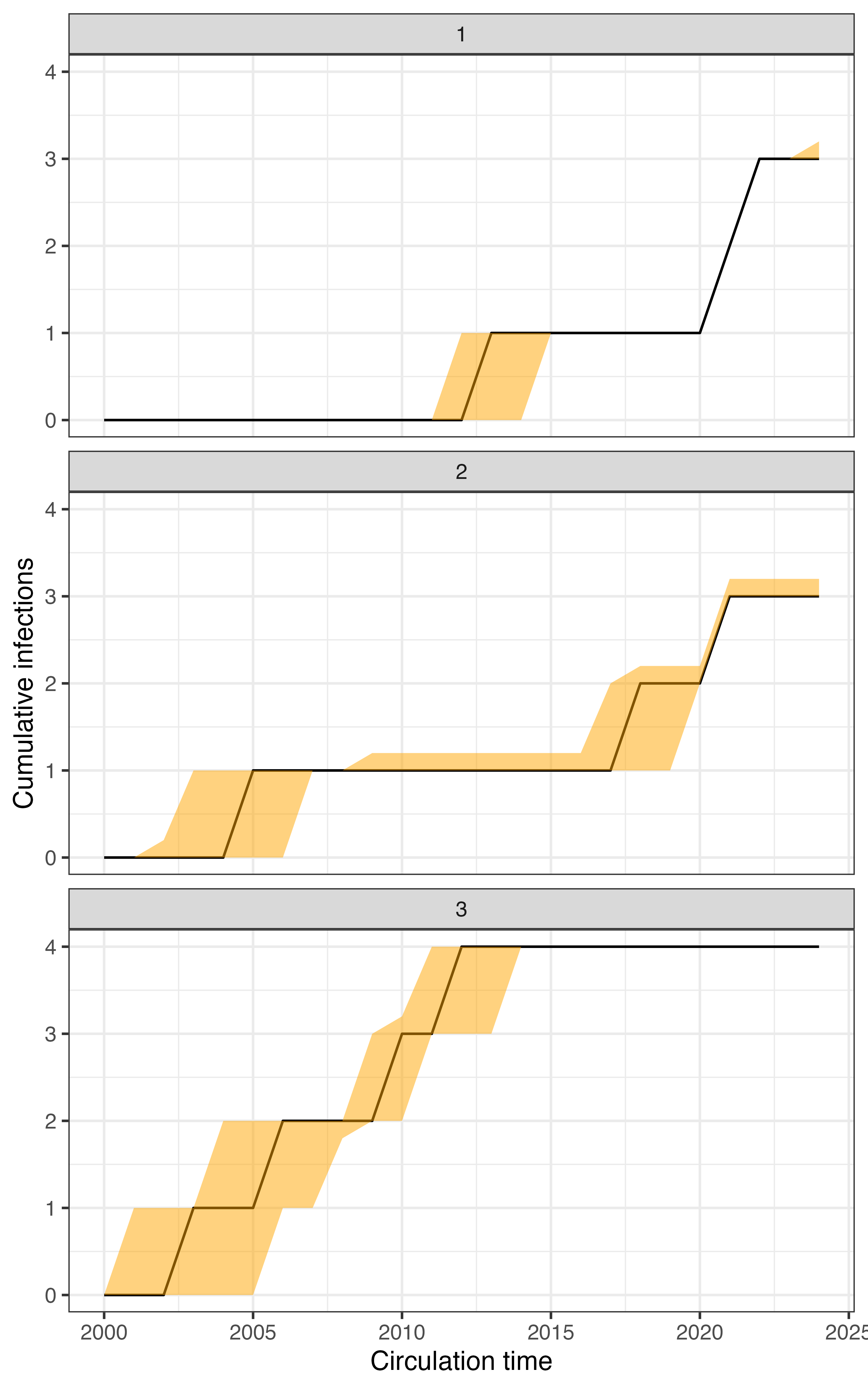

Estimated cumulative infection histories for the first 3 individuals. Line/shaded region shows posterior median/95% CrI on the cumulative number of infections over time.

print(p_cumu_infs[[2]])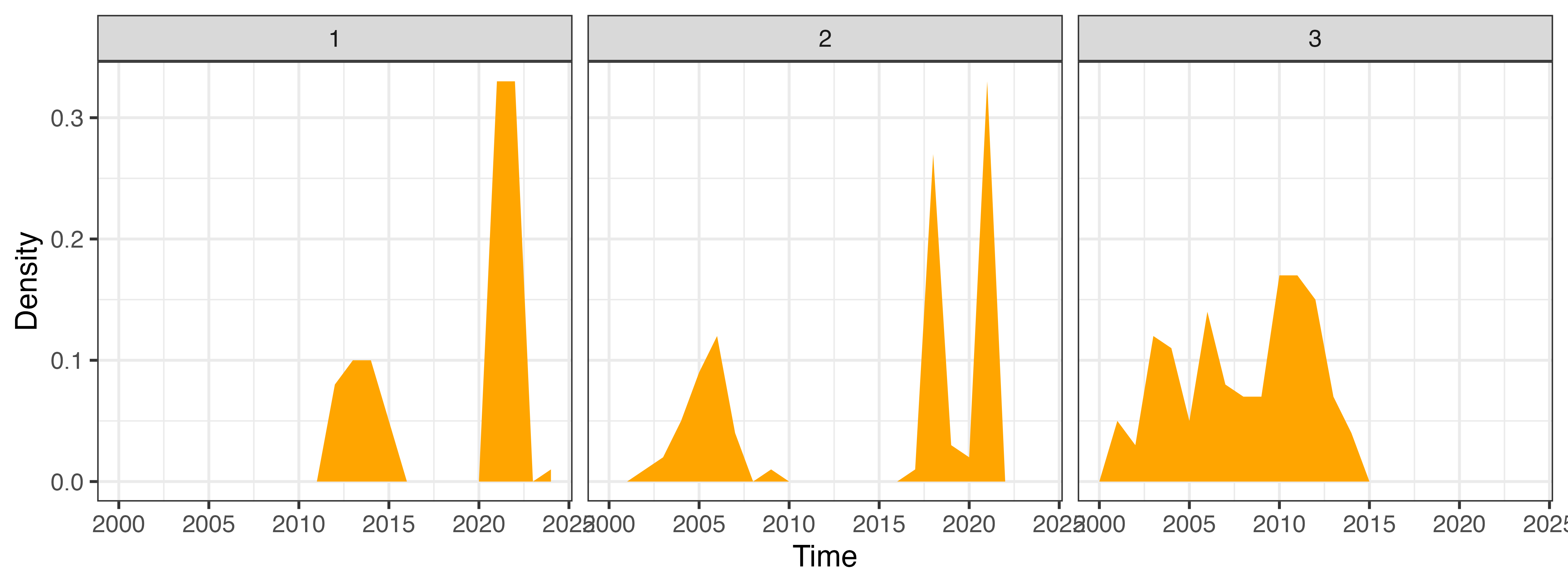

Estimated infection histories for the first 3 individuals. Orange shaded regions show the posterior probability of infection at each time period (x-axis).

Summary

serosolver is a flexible model with many options and outputs. This increases the range of use cases, but also imposes a burden on the user to make a many design decisions and assumptions. Hopefully, this vignette has provided a decent starting point as a new serosolver user. I encourage you to review the case study vignettes to find an example analysis that fits your desired use case, and to use that as a starting point. The other guides provide more detail on advanced features, and if all else fails, do get in touch or leave an issue on the GitHub repository! Good luck!

References

1.

Kucharski AJ, Lessler J, Cummings DAT, Riley S. Timescales of influenza a/H3N2 antibody dynamics. PLOS Biology. 2018;16: 1–19. doi:10.1371/journal.pbio.2004974

2.

Hay JA, Minter A, Ainslie KEC, Lessler J, Yang B, Cummings DAT, et al. An open source tool to infer epidemiological and immunological dynamics from serological data: serosolver. PLOS Computational Biology. 2020;16: e1007840. doi:10.1371/journal.pcbi.1007840

3.

Smith DJ. Mapping the Antigenic and Genetic. 2004;305: 371–376. doi:10.1126/science.1097211