Intro 2: Explanation of observational and antibody kinetics models

David Hodgson

2024-10-18

Introduction

This document explains two critical parts of the model defined in the provided R code:

1. The Observational Model: This component models the observed data, specifying how the measured values relate to the latent (unobserved) processes.
2. The Antibody Kinetics Model: This component models the changes in antibody levels over time, accounting for both natural decay (waning) and infection-induced changes.

---

0. Load the necessary packages

Install these if they are not already installed.

library(devtools)
library(tidyr)
library(dplyr)
library(serojump)
library(patchwork)

1. The Observational Model

Definition

The observational model captures the process by which observed data (IgG in this case) is generated from the underlying system. It defines the relationship between the true (latent) variables and the observed data.

Code Breakdown

obsLogLikelihood <- function(titre_val, titre_est, pars) {
    ll <- dnorm(titre_val, titre_est, pars[1], log = TRUE)
    ll
}

observationalModel <- list(
    names = c("IgG"),
    model = makeModel(
        addObservationalModel("IgG", c("sigma"), obsLogLikelihood)
    ),
    prior = bind_rows(
        add_par_df("sigma", 0.0001, 4, "unif", 0.0001, 4)
    ) # observational model,
)

• names = c("IgG"): The observed biomarker here is IgG, representing some measurement, such as a biomarker (e.g., antibody concentration).

• model = makeModel(...): The model is created using the makeModel function, which defines how the observation model is constructed.

• addObservationalModel("IgG", c("sigma"), obsLogLikelihood): This line adds an observational model for IgG, where the parameter sigma is used to model the noise or uncertainty in the observations. The log-likelihood function (obsLogLikelihood) is used to define how the observations relate to the latent variable.

• prior = bind_rows(...): This block defines the prior distribution for the parameter sigma, which controls the observation noise.

• add_par_df("sigma", 0.0001, 4, "unif", 0.0001, 4): The parameter sigma is given a uniform prior distribution between 0.0001 and 4, indicating that the model expects a certain range of variability in the observed data.

Summary

The observational model defines how the IgG variable is observed with some noise, controlled by sigma. The log-likelihood function helps relate the true underlying values to the observed values, while the prior on sigma assumes uniform uncertainty.

2. The Antibody Kinetics Model

Definition

The antibody kinetics model describes how antibody levels evolve over time in response to different factors, such as infection or natural waning. This model accounts for both natural decay in antibody levels and changes due to infection.

Code Breakdown

Define the antibody kinetic functions

noInfSerumKinetics <- function(titre_est, timeSince, pars) {
    titre_est_new <- titre_est - (pars[1] * titre_est) * (timeSince)
    titre_est_new <- max(titre_est_new, 0)
    titre_est_new
}

infTuenisPower2016 <- function(titre_est, timeSince, pars) {

    y1 <- pars[1]
    t1 <- pars[2]
    r <- pars[3]
    alpha <- pars[4]

    v <- 0.001
    mu <- 1 / t1 * y1

    if (timeSince < t1) {
        titre_est_boost <- exp(mu * timeSince)
    } else {
        titre_est_boost <- exp(y1) * (1 + (r - 1) * exp(y1)^{r - 1} * v * (timeSince - t1)) ^ {-1 / (r - 1)}
    }

    titre_est_log <- titre_est + log(titre_est_boost) * max(0, 1 - titre_est * alpha)
    titre_est_log 
}

Create the antibody kinetics model

abkineticsModel <- list(
    model = makeModel(
        addAbkineticsModel("none", "IgG", "none", c("wane"), noInfSerumKinetics),
        addAbkineticsModel("inf", "IgG", "inf", c("y1_h1", "t1_h1", "r_h1", "s"), infTuenisPower2016)
    ),
    prior = bind_rows(
        add_par_df("y1_h1", 1, 6, "unif",  1, 6),
        add_par_df("t1_h1", 3, 14, "unif", 3, 14),
        add_par_df("r_h1", 1, 5, "unif", 1, 5),
        add_par_df("s", 0, 1, "unif", 0, 1),
        add_par_df("wane", 0, 1, "unif", 0, 1)
    )
)

• model = makeModel(...): The antibody kinetics model is built using makeModel, which defines two different antibody response models.

• addAbkineticsModel("none", "PreF", "none", c("wane"), noInfSerumKinetics): This line models the antibody kinetics when there is no infection. The “PreF” biomarker is modeled with the parameter wane, which represents the natural decay or waning of antibody levels over time. The noInfSerumKinetics function describes this process.

• addAbkineticsModel("inf", "PreF", "inf", c("y1_h1", "t1_h1", "r_h1", "s"), infTuenisPower2016): This line models the antibody kinetics after infection. Several parameters describe the response to infection:

  • y1_h1: Initial antibody level post-infection.
  • t1_h1: Time of peak response.
  • r_h1: Rate of antibody decay post-infection.
  • s: Slope of decay after peak response.
  • infTuenisPower2016: The function governing the infection-induced antibody response.

• prior = bind_rows(...): This block defines prior distributions for the model parameters:

  • y1_h1: Uniform prior between 1 and 6, representing the initial antibody level after infection.
  • t1_h1: Normal prior with mean 14 and standard deviation 3, representing the time to peak response.
  • r_h1: Uniform prior between 1 and 5, representing the rate of antibody decay.
  • s: Uniform prior between 0 and 1, representing the slope of the decay post-infection.
  • wane: Uniform prior between 0 and 1, representing the natural waning of antibody levels over time.

Summary

The antibody kinetics model accounts for the natural waning of antibodies in the absence of infection, as well as the antibody response after infection. Parameters such as y1_h1, t1_h1, and r_h1 govern the kinetics of antibody production and decay. The model uses both uniform and normal priors to specify reasonable ranges for these parameters.

3. Full model definition

This R code defines a serological model using different components such as biomarkers, exposure types, observational and antibody kinetics models, and priors. The code creates a model definitions (modeldefinition) and uses these to create a serological model for data analysis (seroModel).

Step-by-Step Breakdown

Step 1: Define the First Model modeldefinition

Once all the data is loaded in, the first step is to define the model. This includes the biomarkers, exposure types, exposure fitted, observational model, and antibody kinetics model. Then, once the list is created, the createSeroJumpModel function is used to create the serojump model.

# See data_format.Rmd vignette about data input types 

biomarkers <- "IgG"

# Create the data_sero dataframe
data_sero <- data.frame(
  id = c(1, 1, 2, 2, 3, 3),
  time = c(1, 50, 1, 50, 1, 50),
  IgG = c(1.2, 4.4, 1.2, 4.4, 3.0, 3.0)
)

# Define possible exposure types
exposureTypes <- c("none", "inf")

# Create the exposure_data dataframe
exposure_data <- data.frame(
  id = c(1),
  time = c(14),
  exposure_type = c("inf")
)

exposureFitted <- "inf"

# Create the attack_rate_data dataframe
attack_rate_data <- data.frame(
  time = rep(1:25),
  prob = rep(1/25, 25)
)

modeldefinition <- list(
    biomarkers = biomarkers,
    exposureTypes = exposureTypes,
    exposureFitted = exposureFitted,
    observationalModel = observationalModel,
    abkineticsModel = abkineticsModel
)

seroModel <- createSeroJumpModel(data_sero, NULL, modeldefinition)

## OUTLINE OF INPUTTED MODEL
## There are  1  measured biomarkers:  IgG 
## There are  2  exposure types in the study period:  none, inf 
## The fitted exposure type is  inf 
## PRIOR DISTRIBUTIONS 
## Prior parameters of observationalModel are:  sigma 
## Prior parameters of abkineticsModel are:  y1_h1, t1_h1, r_h1, s, wane 
## Exposure rate is not defined over the time period. Defaulting to uniform distribution between 1 and  50 .

4.Pre run sanity plots

Before running the whoel model it is good to check the data and the priors. This can be done using a suit of functions plotPriors function.

p1 <- plotSero(seroModel)
p2 <- plotPriorPredictive(seroModel)
p3 <- plotPriorInfection(seroModel)

p1 / p2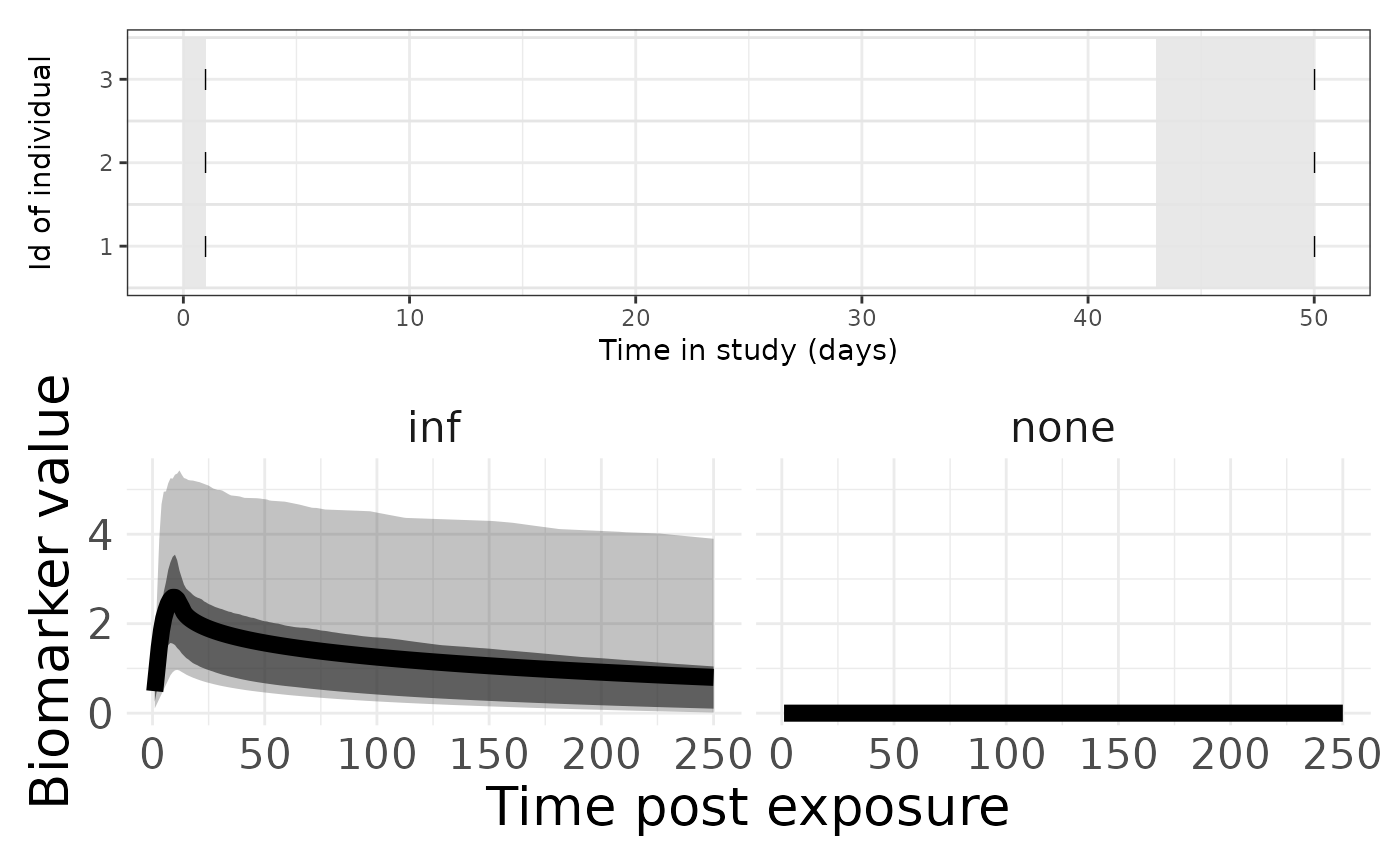

p3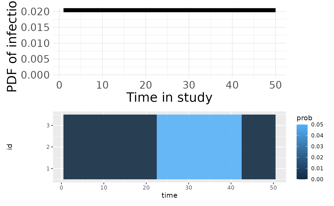

4. Run the model!

Once seroModel is defined, the user can run the model using the runSeroJump function. This function requires the seroModel, settings for the RJ-MCMC algorithm, and information about saving the model outputs.

save_info <- list(
    file_name = "simple",
    model_name = "ex1"
)

# Using more than one core might fail on windows, 
if (.Platform$OS.type == "windows") {
  mc.cores <- 1
} else {
  mc.cores <- 2 # use as many as available, preferably 4.
}

rj_settings <- list(
        numberChainRuns = 4, 
        numberCores = mc.cores,
        iterations = 2000,
        burninPosterior = 1000,
        thin = 1
)

model_summary <- runSeroJump(seroModel, rj_settings, save_info = save_info)

5. Plot the outputs

# Need to have save_info model_summary to run these
plotMCMCDiagnosis(model_summary, save_info = save_info) # plots the convergence diagnosis
plotPostFigs(model_summary, save_info = save_info) #plots some plots of the posteriors

model_summary$post has all the posterior distributions which the user can extract and plot themselves!